Chapter 2 Quantitative phase analysis
This chapter describes methods for quantitative analysis implemented within the powdR package using a range of reproducible examples. Detailed accounts of these methods are provided in Butler and Hillier (2021a) and Butler and Hillier (2021b) and references therein.
One of the most powerful properties of XRPD data is that the intensities of crystalline (e.g., quartz, calcite and gypsum), disordered (e.g., clay minerals), and amorphous (e.g., volcanic glass and organic matter) scattering signals within a diffractogram can be related to the concentrations of these components within the mixture. This principal facilitates the quantification of phase concentrations from XRPD data.
Of the approaches available for quantitative XRPD, the simple Reference Intensity Ratio (RIR) method has consistently proven accurate. A RIR is a measure of the diffracting power of a phase relative to that of a standard (most often corundum, α Al2O3), usually measured in a 50:50 mixture by weight. The RIR of a detectable phase within a mixture is required for its quantification.
As mentioned in Chapter 1, a given diffractogram can be modeled as the sum of pure diffractograms for all detectable phases, each scaled by different amounts (scaling factors). By combining these scaling factors with RIRs, phase concentrations can be calculated. Hereafter this approach is referred to as full pattern summation.
Full pattern summation is particularly suitable for mixtures containing crystalline mineral components in combination with disordered and/or X-ray amorphous phases because the background scattering is also included. Soil is a prime example of such mixtures, where crystalline minerals such as quartz and feldspars can be present in combination with clay minerals (i.e. disordered phases), and organic matter (i.e. amorphous phases). A key component of the full pattern summation approach is the “reference library” containing measured or calculated patterns of the pure phases that may be encountered within the samples. The reference patterns within the library would ideally be measured on the same instrument as the sample, however in some cases this isn’t possible and the data can be harmonised accordingly, at least in some respects. To quantify a given sample, suitable phases from the library are selected that together account for the peaks within the data, and their relative contributions to the observed signal optimised until an appropriate full pattern fit is achieved. This fit is usually refined using least squares optimisation of an objective parameter. The scaled intensities of the optimised patterns are then converted to weight % using the RIRs (see Section 2 in Butler and Hillier 2021a).
2.1 Full pattern summation with powdR
2.1.1 The powdRlib object
A key component of the full pattern summation functions within powdR is the library of reference patterns. These are stored within a powdRlib object created from two basic components using the powdRlib() constructor function. The first component, specified via the xrd_table argument of powdRlib(), is a data frame of the count intensities of the reference patterns, with their 2θ axis as the first column. The column for a given reference pattern must be named using a unique identifier (a phase ID). An example of such a format is provided in the minerals_xrd data:
library(powdR)

data(minerals_xrd)

head(minerals_xrd)
## tth QUA.1 QUA.2 FEL ORT SAN ALB OLI DOL.1 DOL.2 ILL KAO GOE.1 GOE.2 ORG
## 1 4.00973 69 91 546 599 638 308 343 268 362 3078 525 3549 10000 3225
## 2 4.04865 69 92 524 570 609 294 332 256 345 2960 500 3511 9592 3180
## 3 4.08757 64 86 505 555 582 286 328 250 343 2888 486 3401 9323 3135
## 4 4.12649 64 83 512 543 558 277 310 247 327 2753 474 3290 9042 3092
## 5 4.16541 62 83 478 518 536 275 304 241 318 2718 478 3194 9248 3050
## 6 4.20433 60 81 459 514 517 261 298 228 314 2720 447 3113 8557 3010The second component required to build a powdRlib object, specified via the phases_table argument of powdRlib(), is a data frame containing 3 columns. The first column is a string of unique ID’s corrensponding to the names of each reference pattern in the data provided to the xrd_table argument outlined above. The second column is the name of the phase group that this reference pattern belongs to (e.g. quartz, plagioclase, Illite etc). The third column is the reference intensity ratio (RIR) of that reference pattern (relative to a known standard, usually corundum). An example of the format required for the phases_table argument of powRlib() is provided in the minerals_phases data.
data(minerals_phases)

minerals_phases
## phase_id phase_name rir
## 1 QUA.1 Quartz 4.62
## 2 QUA.2 Quartz 4.34
## 3 FEL K-feldspar 0.75
## 4 ORT K-feldspar 1.03
## 5 SAN K-feldspar 0.93
## 6 ALB Plagioclase 1.31
## 7 OLI Plagioclase 1.06
## 8 DOL.1 Dolomite 2.35
## 9 DOL.2 Dolomite 2.39
## 10 ILL Illite 0.22
## 11 KAO Kaolinite 0.91
## 12 GOE.1 Goethite 0.93
## 13 GOE.2 Goethite 0.37
## 14 ORG Organic-Matter 0.07Crucially when building the powdRlib object, all phase ID’s in the first column of the phases_table must match the column names of the xrd_table (excluding the name of the first column which is the 2θ axis), for example.
identical(names(minerals_xrd[-1]),
          minerals_phases$phase_id)
## [1] TRUEOnce created, powdRlib objects can easily be visualised using the associated plot() method (see ?plot.powdRlib), which accepts the arguments wavelength, refs and interactive that are used to specify the X-ray wavelength, the reference patterns to plot, and the output format, respectively. In all cases where plot() is used in this chapter, the use of interactive = TRUE in the function call will produce an interactive html graph that can be viewed in RStudio or a web browser.
my_lib <- powdRlib(minerals_xrd, minerals_phases)

plot(my_lib, wavelength = "Cu",
     refs = c("ALB", "DOL.1",
              "QUA.1", "GOE.2"),
     interactive = FALSE)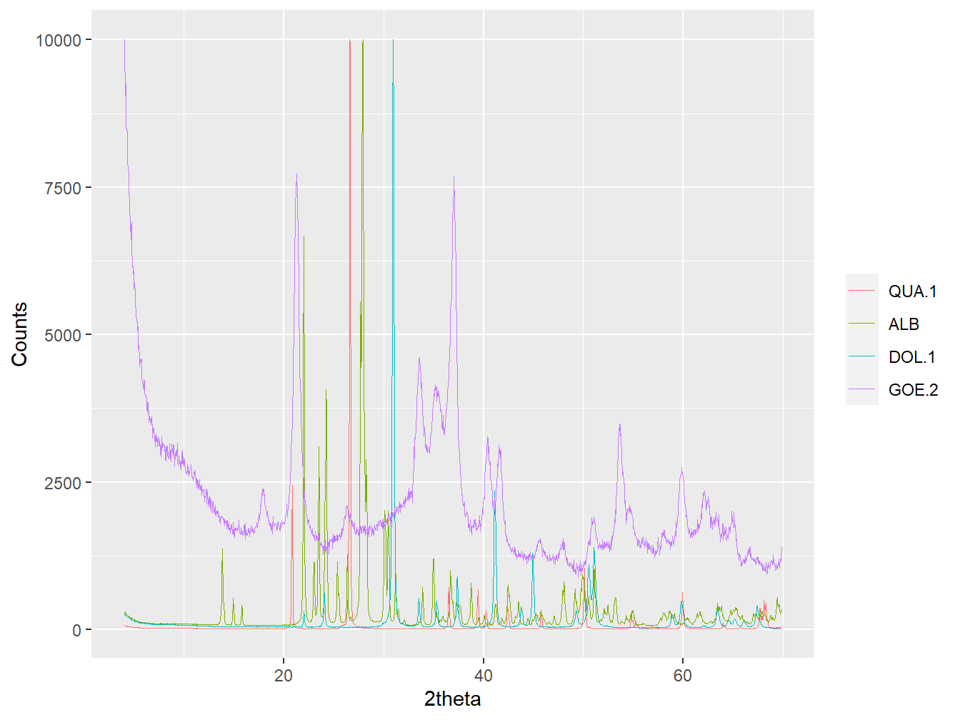
Figure 2.1: Plotting selected reference patterns from a powdRlib object.
2.1.1.1 Pre-loaded powdRlib objects
There are two powdRlib objects provided as part of the powdR package. The first is minerals [accessed via data(minerals)], which is a simple and low resolution library designed to facilitate fast computation of basic examples. The second is rockjock [accessed via data(rockjock)], which is a comprehensive library of 169 reference patterns covering most phases that might be encountered in geological and soil samples. The rockjock library in powdR uses data from the original RockJock program (Eberl 2003) thanks to the permission of Dennis Eberl. In rockjock, each reference pattern from the original RockJock program has been scaled to a maximum intensity of 10000 counts, and the RIRs normalised relative to Corundum. All rockjock data were analysed using Cu K\(\alpha\) radiation. The final library is afsis [accessed via data(minerals)], which contains 21 reference patterns measured on a Bruker D2 phaser as part of the XRPD data analysis undertaken for Africa Soil Information Service Sentinel Site programme.
To accompany the rockjock reference library, a list of eight synthetic mixtures from the original RockJock program (Eberl 2003) are also included in powdR in the rockjock_mixtures data [accessed via data(rockjock_mixtures)], and the known compositions of these mixtures provided in the rockjock_weights data [accessed via data(rockjock_weights)].
2.1.1.2 Subsetting a powdRlib object
Occasionally it may be useful to subset a reference library to a smaller selection. This can be achieved using subset(), which for powdRlib objects accepts three arguments; x, refs and mode (see ?subset.powdRlib). The x argument specifies the powdRlib object to be subset, refs specifies the ID’s and/or names of phases to select, and mode specifies whether these phases are kept (mode = "keep") or removed (mode = "remove").
data(rockjock)

#Have a look at the phase ID's in rockjock
rockjock$phases$phase_id[1:10]
## [1] "CORUNDUM" "BACK_POS"
## [3] "BACK_NEG" "QUARTZ"
## [5] "ORDERED_MICROCLINE" "INTERMEDIATE_MICROCLINE"
## [7] "SANIDINE" "ORTHOCLASE"
## [9] "ANORTHOCLASE" "ALBITE_CLEAVELANDITE"#Remove reference patterns from rockjock
rockjock_1 <- subset(rockjock,
refs = c("ALUNITE", #phase ID
"AMPHIBOLE", #phase ID
"ANALCIME", #phase ID
"Plagioclase"), #phase name
mode = "remove")
#Check number of reference patterns remaining in library
nrow(rockjock_1$phases)## [1] 157#Keep certain reference patterns of rockjock
rockjock_2 <- subset(rockjock,
refs = c("ALUNITE", #phase ID
"AMPHIBOLE", #phase ID
"ANALCIME", #phase ID
"Plagioclase"), #phase name
mode = "keep")
#Check number of reference patterns remaining
nrow(rockjock_2$phases)## [1] 112.1.1.3 Interpolating and merging powdRlib objects
Two powdRlib objects from different instruments can be interpolated and then merged using the interpolate and merge methods (see ?interpolate.powdRlib and merge.powdRlib), respectively. For example, the minerals library can be merged with the rockjock library following interpolation using:
#Load the minerals library
data(minerals)

#Check the number of reference patterns
nrow(minerals$phases)
## [1] 14#Check the number of reference patterns in rockjock
nrow(rockjock$phases)## [1] 168#interpolate minerals library onto same 2theta as rockjock
minerals_i <- interpolate(minerals,
new_tth = rockjock$tth)
#merge the libraries
merged_lib <- merge(rockjock, minerals_i)
#Check the number of reference patterns in the merged library
nrow(merged_lib$phases)## [1] 182In simpler cases where two libraries are already on the same 2θ axis and were measured using the same instrumental parameters, only the use of merge() would be required.
#Load the afsis library
data(afsis)

identical(rockjock$tth, afsis$tth)
## [1] TRUErockjock_afsis <- merge(rockjock, afsis)2.1.2 Full pattern summation with fps()
Once you have a powdRlib reference library and diffractogram(s) loaded into R, you have everything needed for quantitative analysis via full pattern summation. Full pattern summation in powdR is provided via the fps() function, whilst an automated version is provided in afps(). Details of the equations and routines implemented in fps() and afps() are provided in Butler and Hillier (2021a) and Butler and Hillier (2021b).
fps() is specifically applied to powdRlib objects, and accepts a wide range of arguments that are detailed in the package documentation (see ?fps.powdRlib). Here the rockjock and rockjock_mixtures data will be used to demonstrate the main features of fps() and the various ways in which it can be used.
2.1.2.1 Full pattern summation with an internal standard
Often samples are prepared for XRPD analysis with an internal standard of known concentration. If this is the case, then the std and std_conc arguments of fps() can be used to define the internal standard and its concentration (in weight %), respectively, which is then used in combination with the reference intensity ratios to compute phase concentrations. For example, all samples in the rockjock_mixtures data were prepared with 20 % corundum as the added internal standard, thus this can be specified using std = "CORUNDUM" and std_conc = 20 in the call to fps(). In addition, setting the omit_std argument to TRUE makes sure that the internal standard concentration will be omitted from the output and the phase concentrations recomputed accordingly. In such cases the phase specified as the internal standard can also be used in combination with the value specified in the align argument to ensure that the measured diffractogram is appropriately aligned on the 2θ axis using the alignment approach outlined above. These principles are used in the example below, which passes the following seven arguments to fps():
libis used to define thepowdRlibobject containing the reference patterns and their RIRs.smplis used to defined the data frame orXYobject containing the sample diffractogram.refsis used to define a string of phase IDs (lib$phases$phase_id) and/or phase names (lib$phases$phase_names) of the reference patterns to be used in the fitting process.stdis used to define the phase ID of the reference pattern to be used as the internal standard.std_concis used to define the concentration of the internal standard in weight %.omit_stdis used to define whether the internal standard is omitted from the output and phase concentrations recomputed accordingly.alignis used to define the maximum positive or negative shift in 2θ that is permitted during alignment of the sample to the reference pattern that is specified in thestdargument.
data(rockjock_mixtures)

fit1 <- fps(lib = rockjock,
            smpl = rockjock_mixtures$Mix1,
            refs = c("ORDERED_MICROCLINE",
                     "Plagioclase",
                     "KAOLINITE_DRY_BRANCH",
                     "MONTMORILLONITE_WYO",
                     "ILLITE_1M_RM30",
                     "CORUNDUM"),
            std = "CORUNDUM",
            std_conc = 20,
            omit_std = TRUE,
            align = 0.3)
##
## -Aligning sample to the internal standard
## -Interpolating library to same 2theta scale as aligned sample
## -Optimising...
## -Removing negative coefficients and reoptimising...
## -Removing negative coefficients and reoptimising...
## -Computing phase concentrations
## -Using internal standard concentration of 20 % to compute phase concentrations
## -Omitting internal standard from phase concentrations
## ***Full pattern summation complete***Once computed, the fps() function produces a powdRfps object, which is a bundle of data in list format that contains the outputs (see ?fps.powdRlib).
summary(fit1)## Length Class Mode
## tth 2989 -none- numeric
## fitted 2989 -none- numeric
## measured 2989 -none- numeric
## residuals 2989 -none- numeric
## phases 4 data.frame list
## phases_grouped 2 data.frame list
## obj 3 -none- numeric
## weighted_pure_patterns 7 data.frame list
## coefficients 7 -none- numeric
## inputs 16 -none- listThe phase concentrations can be accessed in the phases data frame of the powdRfps object:
fit1$phases## phase_id phase_name rir phase_percent
## 1 CORUNDUM Corundum 1.0000000 NA
## 2 ORDERED_MICROCLINE K-feldspar 0.9654312 3.777500
## 3 ANDESINE Plagioclase 0.8206422 4.660500
## 4 LABRADORITE Plagioclase 0.8113040 20.397000
## 5 KAOLINITE_DRY_BRANCH Kaolinite 0.5812875 14.654375
## 6 ILLITE_1M_RM30 Illite 0.2768664 7.666375
## 7 MONTMORILLONITE_WYO Smectite (Di) 0.3202779 50.955000Further, notice that if the concentration of the internal standard is specified then the phase concentrations do not necessarily sum to 100 % because each phase is quantified with respect to the internal standard:
sum(fit1$phases$phase_percent, na.rm = TRUE)## [1] 102.1108Unlike other software where only certain phases can be used as an internal standard, any phase can be defined in powdR. For example, the rockjock_mixtures$Mix5 sample contains 20 % quartz (see data(rockjock_weights)), thus adding "QUARTZ" as the std argument results in this reference pattern becoming the internal standard instead.
fit2 <- fps(lib = rockjock,
            smpl = rockjock_mixtures$Mix5,
            refs = c("ORDERED_MICROCLINE",
                     "Plagioclase",
                     "KAOLINITE_DRY_BRANCH",
                     "MONTMORILLONITE_WYO",
                     "CORUNDUM",
                     "QUARTZ"),
            std = "QUARTZ",
            std_conc = 20,
            omit_std = TRUE,
            align = 0.3)
##
## -Aligning sample to the internal standard
## -Interpolating library to same 2theta scale as aligned sample
## -Optimising...
## -Removing negative coefficients and reoptimising...
## -Removing negative coefficients and reoptimising...
## -Computing phase concentrations
## -Using internal standard concentration of 20 % to compute phase concentrations
## -Omitting internal standard from phase concentrations
## ***Full pattern summation complete***fit2$phases## phase_id phase_name rir phase_percent
## 1 CORUNDUM Corundum 1.0000000 24.893750
## 2 QUARTZ Quartz 3.5404393 NA
## 3 ORDERED_MICROCLINE K-feldspar 0.9654312 39.810500
## 4 ANORTHOCLASE Plagioclase 0.5804293 3.597250
## 5 ANDESINE Plagioclase 0.8206422 2.626125
## 6 LABRADORITE Plagioclase 0.8113040 3.474375
## 7 ANORTHITE Plagioclase 0.5294816 2.744125
## 8 KAOLINITE_DRY_BRANCH Kaolinite 0.5812875 5.332125
## 9 MONTMORILLONITE_WYO Smectite (Di) 0.3202779 12.902250sum(fit2$phases$phase_percent, na.rm = TRUE)## [1] 95.3805It’s also possible to “close” the mineral composition so that the weight percentages sum to 100. This can be achieved in two ways:
- By defining
closed = TRUEin thefps()function call. - By applying the
close_quant()function to thepowdRfpsoutput.
For example, the phase composition in fit2 created above can be closed using:
fit2c <- close_quant(fit2)

sum(fit2c$phases$phase_percent, na.rm = TRUE)
## [1] 1002.1.2.2 Full pattern summation without an internal standard
In cases where an internal standard is not added to a sample, phase quantification can be achieved by assuming that all detectable phases can be identified and that they sum to 100 weight %. By setting the std_conc argument of fps() to NA, or leaving it out of the function call, it will be assumed that the sample has been prepared without an internal standard and the phase concentrations computed accordingly.
fit3 <- fps(lib = rockjock,
            smpl = rockjock_mixtures$Mix1,
            refs = c("ORDERED_MICROCLINE",
                     "Plagioclase",
                     "KAOLINITE_DRY_BRANCH",
                     "MONTMORILLONITE_WYO",
                     "ILLITE_1M_RM30",
                     "CORUNDUM"),
            std = "CORUNDUM",
            align = 0.3)
##
## -Aligning sample to the internal standard
## -Interpolating library to same 2theta scale as aligned sample
## -Optimising...
## -Removing negative coefficients and reoptimising...
## -Removing negative coefficients and reoptimising...
## -Computing phase concentrations
## -Internal standard concentration unknown. Assuming phases sum to 100 %
## ***Full pattern summation complete***In this case the phase specified in the std argument is only used for 2θ alignment, and is always included in the computed phase concentrations.
fit3$phases## phase_id phase_name rir phase_percent
## 1 CORUNDUM Corundum 1.0000000 19.6679
## 2 ORDERED_MICROCLINE K-feldspar 0.9654312 2.9718
## 3 ANDESINE Plagioclase 0.8206422 3.6665
## 4 LABRADORITE Plagioclase 0.8113040 16.0466
## 5 KAOLINITE_DRY_BRANCH Kaolinite 0.5812875 11.5288
## 6 ILLITE_1M_RM30 Illite 0.2768664 6.0313
## 7 MONTMORILLONITE_WYO Smectite (Di) 0.3202779 40.0871Furthermore, the phase concentrations computed using this approach will always sum to 100 %.
sum(fit3$phases$phase_percent)## [1] 1002.1.2.3 Full pattern summation with data harmonisation
It is usually recommended that the reference library used for full pattern summation is measured on the same instrument as the sample using an identical 2θ range and resolution, along with other identical configurations of the instrument. In some cases this is not feasible, and the reference library patterns may be from a different instrument to the sample. To allow for seamless use of samples and libraries from different instruments (measured using the same X-ray wavelength), fps() contains a logical harmonise argument (default = TRUE). When the sample and library contain non-identical 2θ axes, harmonise = TRUE will convert the data onto the same axis by determining the overlapping 2θ range and interpolating to the coarsest resolution available. This type of approach may produce results that are acceptable and fit for purpose, but if the best accuracy is required then a library of standard patterns collected on the instrument used to run the unknown samples is the recommended approach.
#Create a sample with a shorter 2theta axis than the library
Mix1_short <- subset(rockjock_mixtures$Mix1, tth > 10 & tth < 55)

#Reduce the resolution by selecting only odd rows of the data
Mix1_short <- Mix1_short[seq(1, nrow(Mix1_short), 2),]

fit4 <- fps(lib = rockjock,
            smpl = Mix1_short,
            refs = c("ORDERED_MICROCLINE",
                     "Plagioclase",
                     "KAOLINITE_DRY_BRANCH",
                     "MONTMORILLONITE_WYO",
                     "ILLITE_1M_RM30",
                     "CORUNDUM"),
            std = "CORUNDUM",
            align = 0.3)
##
## -Harmonising library to the same 2theta resolution as the sample
## -Aligning sample to the internal standard
## -Interpolating library to same 2theta scale as aligned sample
## -Optimising...
## -Removing negative coefficients and reoptimising...
## -Removing negative coefficients and reoptimising...
## -Computing phase concentrations
## -Internal standard concentration unknown. Assuming phases sum to 100 %
## ***Full pattern summation complete***fit4$phases## phase_id phase_name rir phase_percent
## 1 CORUNDUM Corundum 1.0000000 19.5826
## 2 ORDERED_MICROCLINE K-feldspar 0.9654312 3.1967
## 3 ANDESINE Plagioclase 0.8206422 4.2983
## 4 LABRADORITE Plagioclase 0.8113040 16.4326
## 5 ANORTHITE Plagioclase 0.5294816 0.1007
## 6 KAOLINITE_DRY_BRANCH Kaolinite 0.5812875 12.9506
## 7 ILLITE_1M_RM30 Illite 0.2768664 8.1800
## 8 MONTMORILLONITE_WYO Smectite (Di) 0.3202779 35.25852.1.3 Automated full pattern summation with afps()
The selection of suitable reference patterns for full pattern summation can often be challenging and time consuming. An attempt to automate this process is provided in the afps() function, which can select appropriate reference patterns from a reference library and subsequently exclude reference patterns based on limit of detection estimates. Such an approach is considered particularly advantageous when quantifying XRPD datasets that display considerable mineralogical variation such as the Reynolds Cup samples. Detailed accounts of the afps() function are provided in Butler and Hillier (2021a) and Butler and Hillier (2021b).
All of the principles and arguments outlined above for the fps() function apply to the use of afps(). However, when usingafps()`, there are a few additional arguments that need to be defined:
forceis used to specify phase IDs (lib$phases$phase_id) or phase names (lib$phases$phase_name) that must be retained in the output, even if their concentrations are estimated to be below the limit of detection or negative.lodis used to define the limit of detection (LOD; in weight %) of the phase specified as the internal standard in thestdargument. This limit of detection for the define phase is then used in combination with the RIRs to estimate the LODs of all other phases.amorphousis used to specify which, if any, phases should be treated as amorphous. This is used because the assumptions used to estimate the LODs of crystalline and disordered phases are not appropriate for amorphous phases.amorphous_lodis used to define the LOD (in weight %) of the phases specified in theamorphousargument.
Here the rockjock library, containing 169 reference patterns, will be used to quantify one of the samples in the rockjock_mixtures data. Note that when using afps(), omission of the refs argument in the function call will automatically result in all phases from the reference library being used in the fitting process.
#Produce the fit
a_fit1 <- afps(lib = rockjock,
               smpl = rockjock_mixtures$Mix1,
               std = "CORUNDUM",
               align = 0.3,
               lod = 1)
##
## -Using all reference patterns in the library
## -Aligning sample to the internal standard
## -Interpolating library to same 2theta scale as aligned sample
## -Applying non-negative least squares
## -Optimising...
## -Removing negative coefficients and reoptimising...
## -Calculating detection limits
## -Removing phases below detection limit
## -Reoptimising after removing crystalline phases below the limit of detection
## -Computing phase concentrations
## -Internal standard concentration unknown. Assuming phases sum to 100 %
## ***Automated full pattern summation complete***Once computed, the afps function produces a powdRafps object, which is a bundle of data in list format that contains the outputs (see ?afps.powdRlib). When large libraries such a rockjock are used to quantify a given sample, the resulting output is likely contain several different reference patterns for a given mineral, for example:
table(a_fit1$phases$phase_name)##
## Background Corundum Illite K-feldspar Kaolinite
## 1 1 2 1 1
## Plagioclase Smectite (Di)
## 3 2Illustrates that the resulting output contains 2 reference patterns for both illite and smectite, 3 patterns for plagioclase, and 1 pattern for each of the other phases selected by afps()'. This information is grouped together and summed in thephases_groupeddata frame within thepowdRafps` object:
a_fit1$phases_grouped## phase_name phase_percent
## 1 Corundum 19.2449
## 2 Background 0.0001
## 3 K-feldspar 2.6398
## 4 Plagioclase 19.2431
## 5 Kaolinite 10.8828
## 6 Smectite (Di) 40.0788
## 7 Illite 7.9105Grouping of phases like this is a powerful approach to obtain better fits to the minerals present in a given sample, and is advantageous even for minerals like quartz, where some combination of several quartz standards may produce a better fit that a single standard. Note also that the “background” phase in the output is simply a horizontal line that can account for shifts in background intensity, which can be useful to use in some cases, but most especially when working with data and libraries from different instruments. In the rockjock data, the background patterns have been given an exceptionally high RIR so that their quantified concentrations are effectively zero.
2.1.4 Additional fps() and afps() functionality
2.1.4.1 Shifting of reference patterns
Both fps() and afps() accept a shift argument, which when set to a value greater than zero results in optimisation of a small 2θ shift for each reference pattern in order to improve the quality of the fit. The value supplied to the shift argument defines the maximum (either positive or negative) shift that can be applied to each reference pattern before the shift is reset to zero.
This shifting process is designed to correct for small linear differences in the peak positions of the standards relative to the sample, which may result from a combination of instrumental aberrations, mineralogical variation and/or uncorrected errors in the library patterns. Whilst it provides more accurate results, the process can substantially increase computation time.
2.1.4.2 Regrouping phases in powdRfps and powdRafps objects
Occasionally it can be useful to apply a different grouping structure to the phases quantified within a powdRfps or powdRafps object. This can be achieved using the regroup function (see ?regroup.powdRfps and ?regroup.powdRafps):
#Load the rockjock regrouping structure
data(rockjock_regroup)

#Check the first 6 rows of the data
head(rockjock_regroup)
## phase_id phase_name_grouped phase_name_grouped2
## 1 CORUNDUM Corundum Non-clay
## 2 BACK_POS Background Background
## 3 BACK_NEG Background Background
## 4 QUARTZ Quartz Non-clay
## 5 ORDERED_MICROCLINE K-feldspar Non-clay
## 6 INTERMEDIATE_MICROCLINE K-feldspar Non-clay#Regroup the data in a_fit1 using the coarsest resolution
#(i.e. select columns 1 and 3 from the data)
a_fit1_rg <- regroup(a_fit1, rockjock_regroup[c(1,3)])
#Check the changes made to the data
a_fit1_rg$phases## phase_id phase_name rir phase_percent
## 1 CORUNDUM Non-clay 1.000000e+00 19.2449
## 2 BACK_NEG Background 1.000000e+04 0.0001
## 3 ORDERED_MICROCLINE Non-clay 9.654312e-01 2.6398
## 4 ANDESINE Non-clay 8.206422e-01 3.2496
## 5 LABRADORITE Non-clay 8.113040e-01 15.8851
## 6 BYTOWNITE Non-clay 7.250736e-01 0.1084
## 7 ORD_KAOLINITE Clay 6.684230e-01 10.8828
## 8 CA_MONTMORILLONITE Clay 2.920099e-01 16.1587
## 9 ILLITE_1M_RM30 Clay 2.768664e-01 4.9353
## 10 MONTMORILLONITE_WYO Clay 3.202779e-01 23.9201
## 11 ILLITE_R0_5_PERCENT_I Clay 2.620735e-01 2.9752#Check the new grouped data
a_fit1_rg$phases_grouped## phase_name phase_percent
## 1 Background 0.0001
## 2 Clay 58.8721
## 3 Non-clay 41.12782.2 Plotting powdRfps and powdRafps objects
Plotting results powdRfps and powdRafps objects, derived from fps() and afps(), respectively, is achieved using plot() (see ?plot.powdRfps and ?plot.powdRafps).
plot(a_fit1, wavelength = "Cu", interactive = FALSE)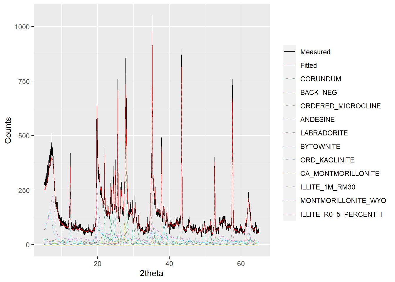
Figure 2.2: Example output from plotting a powdRfps or powdRafps object.
When plotting powdRfps or powdRafps objects the wavelength must be defined because it is required to compute d-spacings that are shown when interactive = TRUE. As with other plotting methods outlined in Section 1.3, interactive ggplotly() outputs can be created using interactive = TRUE.
In addition to above, plotting for powdRfps and powdRafps objects can be further adjusted by the group, mode and xlim arguments. When the group argument is set to TRUE, the patterns within the fit are grouped and summed according to phase names, which can help simplify the plot:
plot(a_fit1, wavelength = "Cu",
     group = TRUE,
     interactive = FALSE)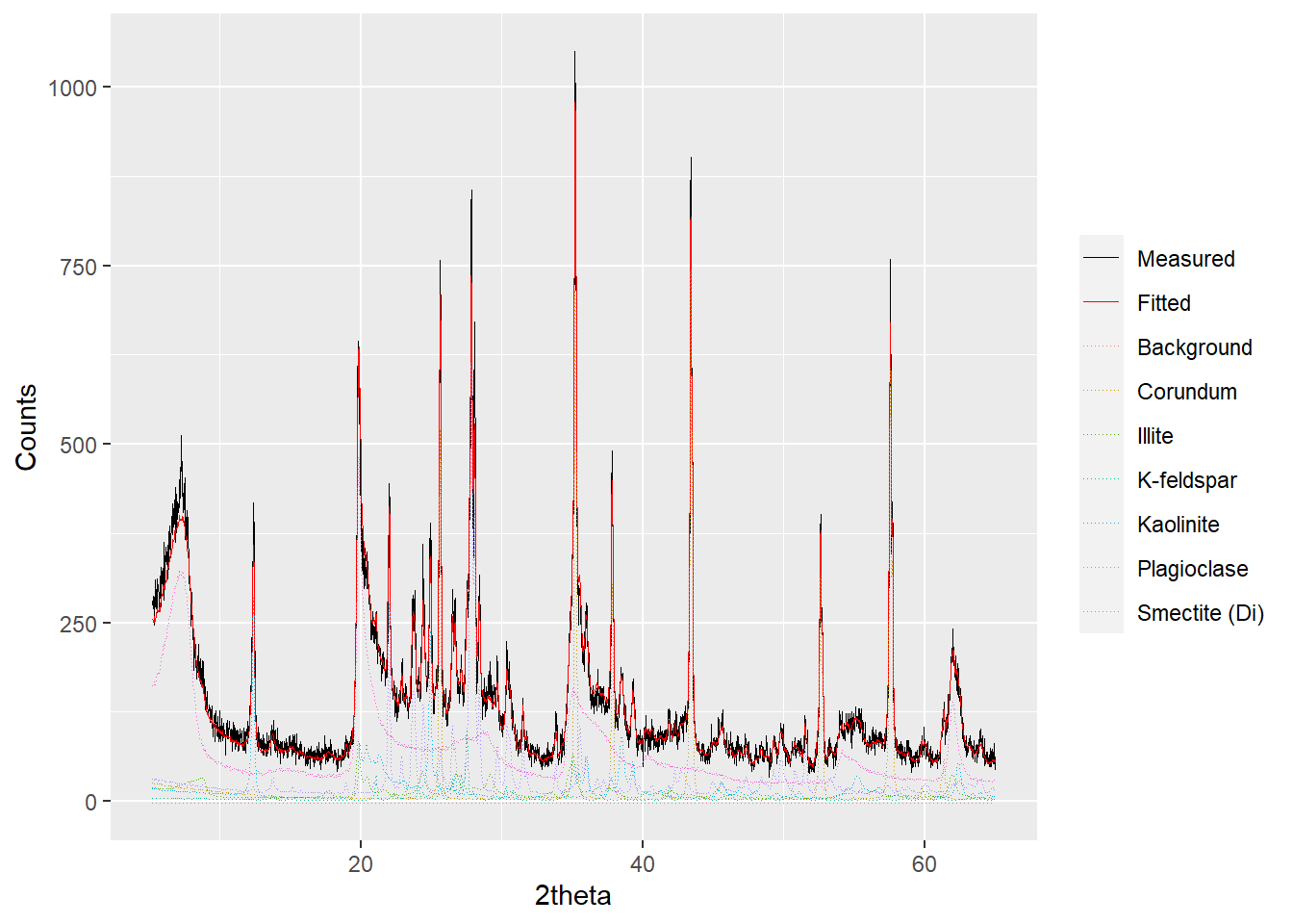
Figure 2.3: Plotting a powdRfps or powdRafps object with the reference patterns grouped.
The mode argument can be one of "fit" (the default), "residuals" or "both", for example:
plot(a_fit1, wavelength = "Cu",
     mode = "residuals",
     interactive = FALSE)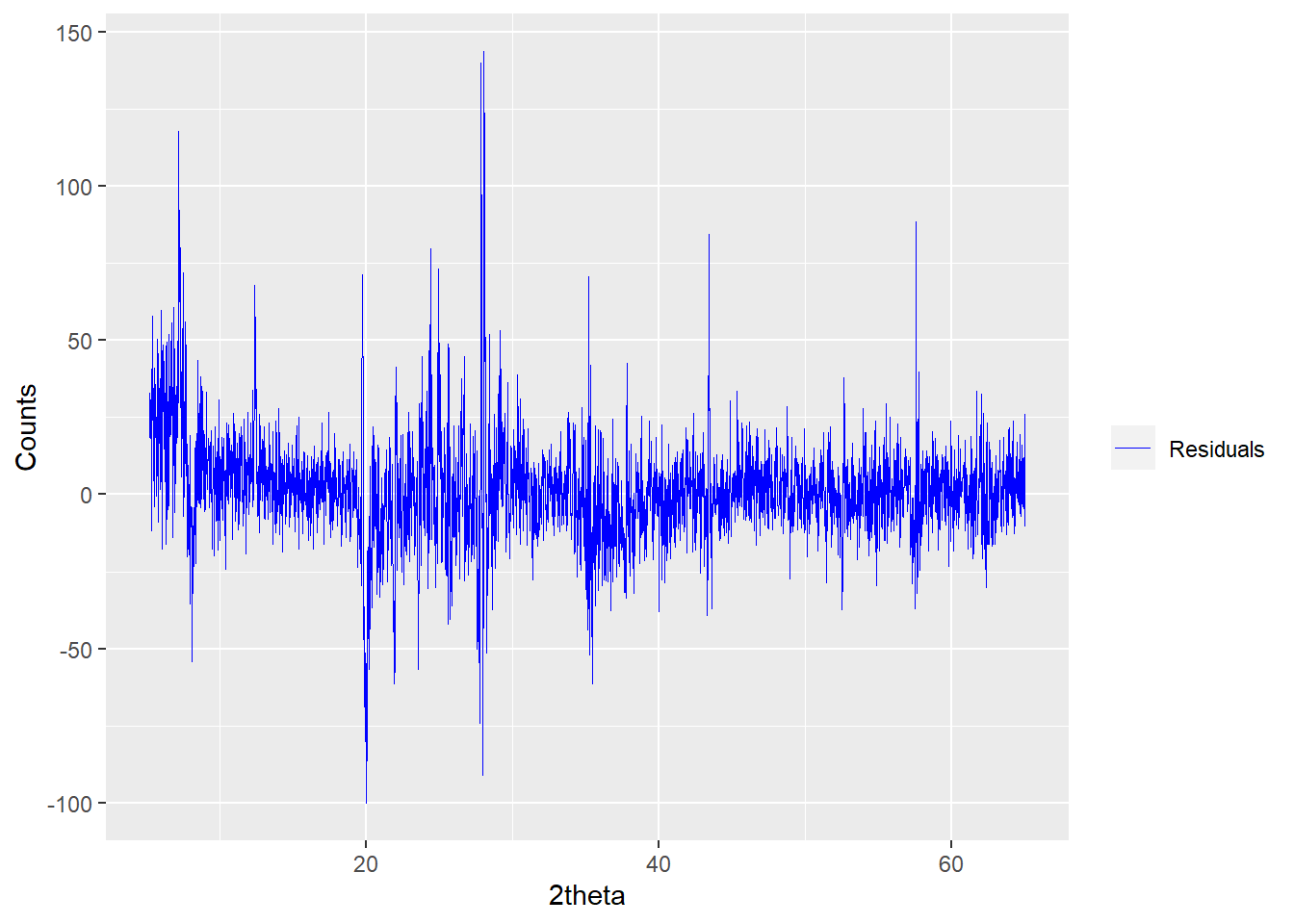
Figure 2.4: Plotting the residuals of a powdRfps or powdRafps object.
or alternatively both the fit and residuals can be plotted using mode = "both" and the 2θ axis restricted using the xlim argument:
plot(a_fit1, wavelength = "Cu",
     mode = "both", xlim = c(20,30),
     interactive = FALSE)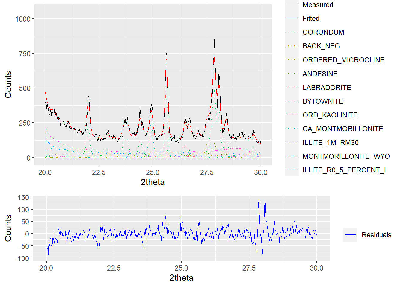
Figure 2.5: Plotting both the fit and residuals of a powdRfps or powdRafps object.
2.3 Quantifying multiple samples
2.3.1 lapply()
The simplest way to quantify multiple samples via either fps() and afps() is by wrapping either of the functions in lapply() and supplying a list of diffractograms. The following example wraps the fps() function in lapply and applies the function to the first three items within the rockjock_mixtures data.
multi_fit <- lapply(rockjock_mixtures[1:3], fps,
                    lib = rockjock,
                    std = "CORUNDUM",
                    refs = c("ORDERED_MICROCLINE",
                             "LABRADORITE",
                             "KAOLINITE_DRY_BRANCH",
                             "MONTMORILLONITE_WYO",
                             "ILLITE_1M_RM30",
                             "CORUNDUM",
                             "QUARTZ"),
                    align = 0.3)
##
## -Aligning sample to the internal standard
## -Interpolating library to same 2theta scale as aligned sample
## -Optimising...
## -Computing phase concentrations
## -Internal standard concentration unknown. Assuming phases sum to 100 %
## ***Full pattern summation complete***
##
## -Aligning sample to the internal standard
## -Interpolating library to same 2theta scale as aligned sample
## -Optimising...
## -Computing phase concentrations
## -Internal standard concentration unknown. Assuming phases sum to 100 %
## ***Full pattern summation complete***
##
## -Aligning sample to the internal standard
## -Interpolating library to same 2theta scale as aligned sample
## -Optimising...
## -Removing negative coefficients and reoptimising...
## -Computing phase concentrations
## -Internal standard concentration unknown. Assuming phases sum to 100 %
## ***Full pattern summation complete***When using lapply in this way, the names of the items within the list or multiXY object supplied to the function are inherited by the output:
identical(names(rockjock_mixtures[1:3]),
          names(multi_fit))
## [1] TRUE2.3.2 Parallel processing
Whilst lapply is a simple way to quantify multiple samples, the computation remains restricted to a single core. Computation time can be reduced many-fold by allowing different cores of your machine to process one sample at a time, which can be achieved using the doParallel and foreach packages:
#Install the foreach and doParallel package
install.packages(c("foreach", "doParallel"))

#load the packages
library(foreach)
library(doParallel)

#Detect number of cores on machine
UseCores <- detectCores()

#Register the cluster using n - 1 cores
cl <- makeCluster(UseCores-1)

registerDoParallel(cl)

#Use foreach loop and %dopar% to compute in parallel
multi_fit <- foreach(i = 1:3) %dopar%
  (powdR::fps(lib = rockjock,
               smpl = rockjock_mixtures[[i]],
               std = "CORUNDUM",
               refs = c("ORDERED_MICROCLINE",
                        "LABRADORITE",
                        "KAOLINITE_DRY_BRANCH",
                        "MONTMORILLONITE_WYO",
                        "ILLITE_1M_RM30",
                        "CORUNDUM",
                        "QUARTZ"),
               align = 0.3))

#name the items in the aquant_parallel list
names(multi_fit) <- names(rockjock_mixtures)[1:3]

#stop the cluster
stopCluster(cl)
Note how the call to fps uses the notation powdR::fps(), which specifies the accessing of the fps() function from the powdR package.
2.4 Summarising mineralogy
When multiple samples are quantified it is often useful to report the phase concentrations of all of the samples in a single table. For a given list of powdRfps and/or powdRafps objects, the summarise_mineralogy() function yields such summary tables, for example:
summarise_mineralogy(multi_fit, type = "grouped", order = TRUE)## sample_id Kaolinite Corundum Plagioclase Smectite (Di) Illite K-feldspar
## 1 Mix1 11.4255 19.6390 18.9222 40.2223 6.0943 3.4771
## 2 Mix2 19.9893 20.1257 34.2955 3.1401 9.8914 7.9668
## 3 Mix3 38.0548 20.1476 NA 3.5897 19.4220 11.0541
## Quartz
## 1 0.2197
## 2 4.5911
## 3 7.7318where type = "grouped" denotes that phases with the same phase_name will be summed together, and order = TRUE specifies that the columns will be ordered from most common to least common (assessed by the sum of each column). Using type = "all" instead would result in tabulation of all phase IDs.
In addition to the quantitative mineral data, three objective parameters that summarise the quality of the fit can be appended to the table via the logical rwp, r and delta arguments.
summarise_mineralogy(multi_fit, type = "grouped", order = TRUE,
                     rwp = TRUE, r = TRUE, delta = TRUE)
## sample_id Kaolinite Corundum Plagioclase Smectite (Di) Illite K-feldspar
## 1 Mix1 11.4255 19.6390 18.9222 40.2223 6.0943 3.4771
## 2 Mix2 19.9893 20.1257 34.2955 3.1401 9.8914 7.9668
## 3 Mix3 38.0548 20.1476 NA 3.5897 19.4220 11.0541
## Quartz Rwp R Delta
## 1 0.2197 0.1193771 0.1165048 39834.67
## 2 4.5911 0.1237287 0.1115322 36910.18
## 3 7.7318 0.1141585 0.1077551 37571.72For each of these parameters, lower values represent a smaller difference between the measured and fitted patterns, and hence are indicative of a better fit. For more information see Section 2.1 in Butler and Hillier (2021b).
2.5 The powdR Shiny app
All above examples showcase the use of R code to carry out full pattern summation. It is also possible to run much of this functionality of powdR via a Shiny web application. This Shiny app can be loaded in your default web browser by running run_powdR(). The resulting application has six tabs:
- Reference Library Builder: Allows you to create and export a
powdRlibreference library from two ‘.csv’ files: one for the XRPD measurements, and the other for the ID, name and reference intensity ratio of each pattern. - Reference Library Viewer: Facilitates quick inspection of the phases within a
powdRlibreference library. - Reference Library Editor: Allows the user to easily subset a
powdRlibreference library . - Full Pattern Summation: A user friendly interface for iterative full pattern summation of single samples using
fps()orafps(). - Results Viewer/Editor: Allows for results from previously saved
powdRfpsandpowdRafpsobjects to be viewed and edited via addition or removal of reference patterns. - Help Provides a series of video tutorials (via YouTube) detailing the use of the powdR Shiny application.