Chapter 4 Cluster analysis of soil XRPD data
This chapter will demonstrate the use of cluster analysis to identify mineral-nutrient relationships in African soils. The examples provided for the cluster analysis use the data presented in Butler et al. (2020) that is hosted here on Mendeley Data. To run the examples in this chapter on your own machine, you will need to download the soil property data in ‘.csv’ format and the XRPD data in a zipped folder of ‘xy’ files. Please simply save these files to your own directory, and unzip the zipped folder containing the ‘.xy’ files. Skip this step if you have already downloaded these files for the examples in Chapter 3,
4.1 Loading packages and data
This chapter will use a number of packages that should already be installed on your machine, but will also use the reshape2 and e1071 packages that may need to be installed if you have not used them before:
#install packages that haven't been used in the course before
install.packages(c("reshape2", "e1071"))
#load the relevant packages
library(reshape2)
library(e1071)
library(leaflet)
library(powdR)
library(ggplot2)
library(plotly)
library(gridExtra)
library(plyr)Once you have loaded the packages and downloaded the data required for this chapter (note that it is the same data as that used in Chapter 3), the data can be loaded into R by modifying the paths in the following code:
#Load the soil property data
props <- read.csv(file = "path/to/your/file/clusters_and_properties.csv")

#Get the full file paths of the XRPD data
xrpd_paths <-  dir("path/to/xrd", full.names = TRUE)

#Load the XRPD data
xrpd <- read_xy(files = xrpd_paths)

#Make sure the data are interpolated onto the same 2theta scale
#as there are small differences within the dataset
xrpd <- interpolate(xrpd, new_tth = xrpd$icr030336$tth)
The resulting loaded data matches that loaded and explored in Chapter 3, with the props data containing a range of geochemical soil properties and the xrpd data containing an XY diffractogram of each sample.
4.2 Principal component analysis
The cluster analysis in this Chapter is applied to principal components of soil XRPD data derived using Principal Component Analysis [PCA; Jolliffe (1986)]. Prior to applying cluster analysis to the XRPD data via this approach, it is important to apply corrections for sample-independent variation such as small 2θ misalignments and/or fluctuations in count intensities. For this example, the pre-treatment routine will be based on that defined in Butler et al. (2020), and will involve alignment, subsetting, square root transformation and mean centering. Together these correct for common experimental aberrations so that the variation in the observed data is almost entirely sample-dependent. The pre-treatment steps used here also match those described in Section 3.3 except for the additional step of square root transforming the data, which acts to reduce the relative intensity of quartz peaks that can often dominate the overall variation in diffraction data because quartz is such a strong diffractor.
Alignment of the data can be carried out using the align_xy() function, which aligns each sample within the dataset to a pure reference pattern, which in this case will be quartz that is omnipresent within the soil dataset:
#load the afsis reference library
data(afsis)

#Extract a quartz pattern from it
quartz <- data.frame(afsis$tth,
                     afsis$xrd$QUARTZ_1_AFSIS)

#Align the xrpd data to this quartz pattern
#using a restricted 2theta range of 10 to 60
xrpd_aligned <- align_xy(xrpd, std = quartz,
                         xmin = 10, xmax = 60,
                         xshift = 0.2)
Aligned data can then be subset to 2θ >= 6 so that the high background at low angles (Figure 3.4) in the data can be removed.
xrpd_aligned_sub <- lapply(xrpd_aligned, subset,
                           tth >= 6)
Following alignment, the remaining data pre-treatment steps (square root transform and mean centering) and the PCA can all be carried out in a single step using the xrpd_pca() function from powdR:
pca <- xrpd_pca(xrpd_aligned_sub,
                mean_center = TRUE,
                root_transform = 2,
                components = 5)

#View the variance explained by the first 5 PCs
pca$eig[1:5,]
## eigenvalue variance.percent cumulative.variance.percent
## Dim.1 32304.1020 81.451846 81.45185
## Dim.2 2073.3848 5.227851 86.67970
## Dim.3 1054.2328 2.658152 89.33785
## Dim.4 731.3746 1.844094 91.18194
## Dim.5 611.6932 1.542329 92.72427From which it can be seen that the first 5 principal components (PCs) of the data account for 93 % of variation in the XRPD data. For simplicity this example will use the first 5 PCs hereafter, which can be plotted against one-another using the following code:
#Define the x-axis components
x <- c(1, 1, 1, 1,
       2, 2, 2,
       3, 3,
       4)

#Define the y-axis components
y <- c(2, 3, 4, 5,
       3, 4, 5,
       4, 5,
       5)

#Create an empty list
p <- list()

#Populate each item in the list using the dimension defined
#in x and y
for (i in 1:length(x)) {

   p[[i]] <- ggplot(data = pca$coords) +
             geom_point(aes_string(x = paste0("Dim.", x[i]),
                                   y = paste0("Dim.", y[i])),
                        shape = 21,
                        size = 3)

}

grid.arrange(grobs = p,
             ncol = 2)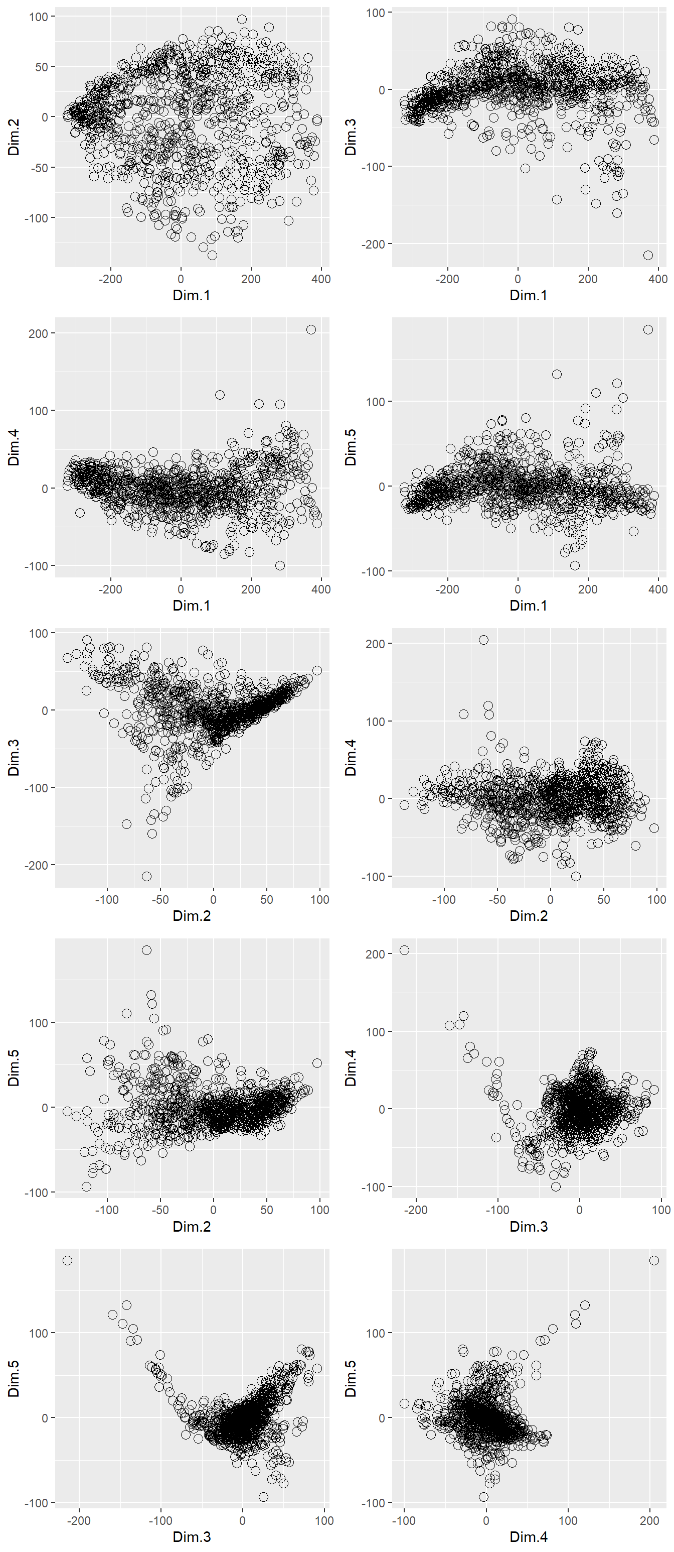
Figure 4.1: The first 5 PCs plotted against one-another
4.2.1 Interpreting principal components
Whilst we’re able to derive that the first 5 PCs explain 93 % of variation in the XRPD data and plot the resulting variables against one-another, we are still not in a position to interpret what the scores actually mean. For example, how do increased/decreased values in Dim.1 reflect mineralogical differences in the soil samples? This interpretation can be achieved by examining the loadings of each PC dimension, for example the loading of Dim.1 can be visualised via:
ggplot(data = pca$loadings) +
  geom_line(aes(x = tth, y = Dim.1)) +
  geom_hline(yintercept = 0)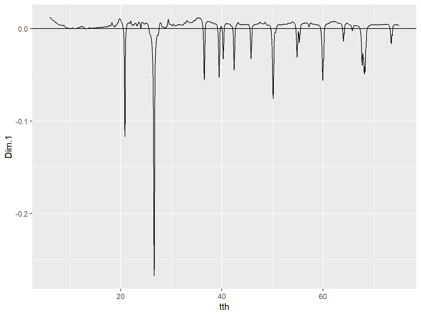
Figure 4.2: The loading of Dim.1.
These loadings represent the weights of each variable that are used when calculating the PCs. In this case, increased values of Dim.1 would result from increased intensity in the regions of the positive peaks of the loading, whereas decreased values of Dim.1 would result from increased intensity in regions of broad but negative peaks. In order to ascertain what these positive and negative features represent, it is possible to apply the full pattern summation principles outlined in Chapter 2 to the loadings.
Whilst full pattern summation for quantitative analysis deals with scaling factors that should only be positive, the loadings of each PC can be modeled in a similar manner by allowing the scaling coefficients to be either positive or negative. Such analysis can be achieved using the fps_lm() function of powdR. This function uses linear regression to compute the scaling factor and allows you to set a p-value that can help omit unnecessary patterns from the fit. Whilst the full pattern summation outlined in Chapter 2 results in phase quantification, fps_lm() is only intended to help with the identification of reference library patterns contributing to a given pattern and therefore does not require or use Reference Intensity Ratios. Below fps_lm() is used to model the loading of Dim.1:
#Load the rockjock library
data(rockjock)

#Merge the rockjock and afsis libraries
rockjock_afsis <- merge(rockjock, afsis)

#All patterns in the library need to be square root transformed
#because this transformation was applied to the soil data
#during the use of xrpd_pca(). In order to avoid errors with the square
#root transforms, any reference pattern with negative counts
#must be removed from the library

remove_index <- which(unlist(lapply(rockjock$xrd, min)) < 0)

rockjock_afsis <- subset(rockjock_afsis,
                         refs = names(rockjock_afsis$xrd)[remove_index],
                         mode = "remove")

#Square root transform the counts
rockjock_afsis_sqrt <- rockjock_afsis
rockjock_afsis_sqrt$xrd <- sqrt(rockjock_afsis_sqrt$xrd)

#Produce a fit using a subset of common soil minerals
dim1_fit <- fps_lm(rockjock_afsis_sqrt,
                   smpl = data.frame(pca$loadings$tth,
                                     pca$loadings$Dim.1),
                   refs = c("Quartz",
                            "Organic matter",
                            "Plagioclase",
                            "K-feldspar",
                            "Goethite",
                            "Illite",
                            "Mica (Di)",
                            "Kaolinite",
                            "Halloysite",
                            "Dickite",
                            "Smectite (Di)",
                            "Smectite (ML)",
                            "Goethite",
                            "Gibbsite",
                            "Amphibole",
                            "Calcite",
                            "Ferrihydrite"),
                     std = "QUARTZ_1_AFSIS",
                     align = 0, #No alignment needed
                     p = 0.01)
##
## -Harmonising sample to the same 2theta resolution as the library
## -Applying linear regression
## -Removing coefficients with p-value greater than 0.01
## -Removing coefficients with p-value greater than 0.01
## -Removing coefficients with p-value greater than 0.01
## ***Full pattern summation complete***plot(dim1_fit, wavelength = "Cu", group = TRUE)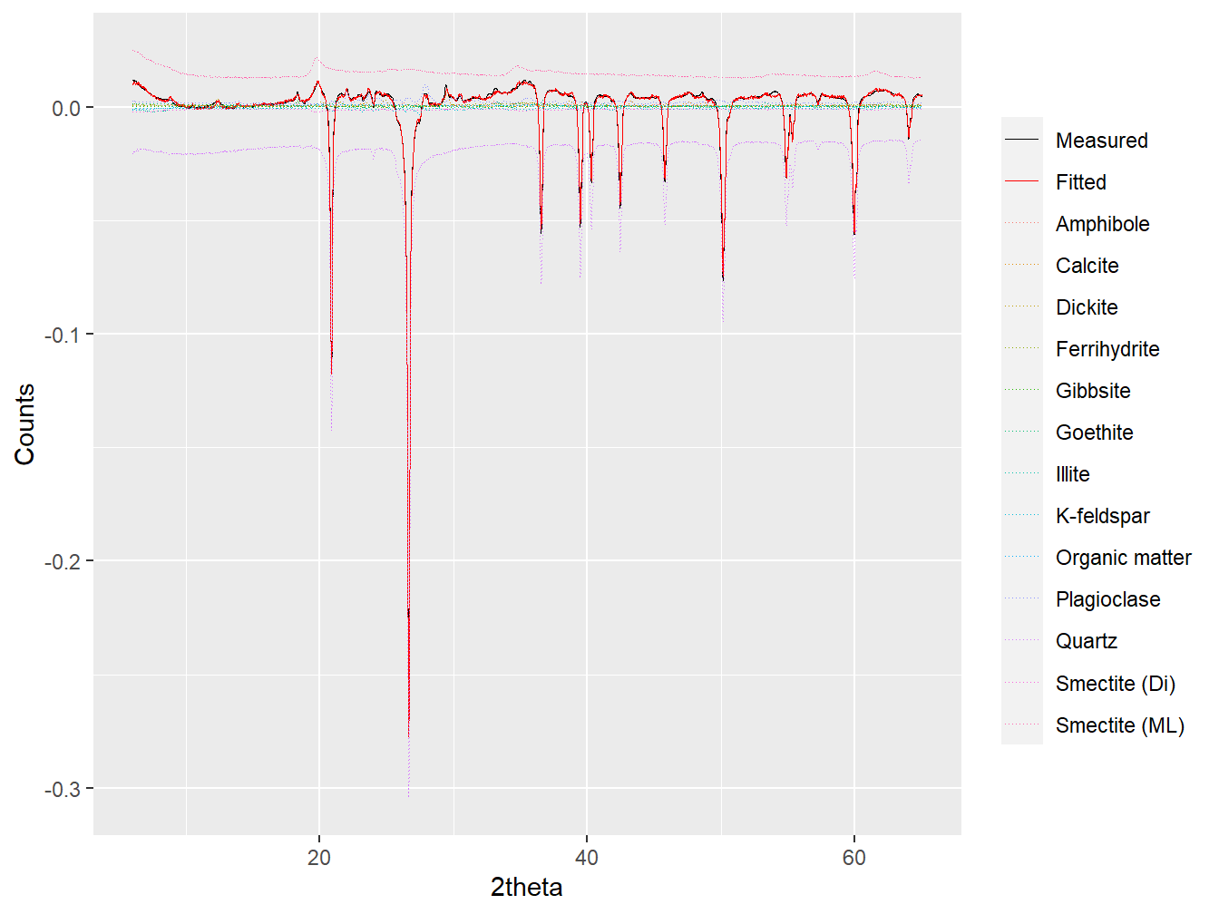
Figure 4.3: Full pattern summation applied to the loading of Dim.1.
dim1_fit$phases_grouped[order(dim1_fit$phases_grouped$coefficient),]## phase_name coefficient
## 11 Quartz -3.081022e-03
## 8 K-feldspar -3.169293e-05
## 12 Smectite (Di) -2.213481e-05
## 9 Organic matter 1.171259e-05
## 7 Illite 1.672584e-05
## 4 Ferrihydrite 1.692329e-05
## 1 Amphibole 2.371968e-05
## 5 Gibbsite 2.664863e-05
## 6 Goethite 3.529204e-05
## 3 Dickite 3.673291e-05
## 2 Calcite 6.545188e-05
## 10 Plagioclase 1.048826e-04
## 13 Smectite (ML) 2.813015e-04By interpreting the plot (particularly using interactive = TRUE) and the coefficients it can be seen that more negative Dim.1 scores are promoted by increased intensity of quartz peaks, whereas more positive Dim.1 scores are promoted by increased intensity of Smectite peaks. Dim.1 can therefore be interpreted to broadly represent the acid-basic gradient of soil parent materials. Applying the same analysis to the loading of Dim.2 yields a very different interpretation:
dim2_fit <- fps_lm(rockjock_afsis_sqrt,
                   smpl = data.frame(pca$loadings$tth,
                                     pca$loadings$Dim.2),
                   refs = c("Quartz",
                            "Organic matter",
                            "Plagioclase",
                            "K-feldspar",
                            "Goethite",
                            "Illite",
                            "Mica (Di)",
                            "Kaolinite",
                            "Halloysite",
                            "Dickite",
                            "Smectite (Di)",
                            "Smectite (ML)",
                            "Goethite",
                            "Gibbsite",
                            "Amphibole",
                            "Calcite",
                            "Ferrihydrite"),
                     std = "QUARTZ_1_AFSIS",
                     align = 0, #No alignment needed
                     p = 0.01)
##
## -Harmonising sample to the same 2theta resolution as the library
## -Applying linear regression
## -Removing coefficients with p-value greater than 0.01
## -Removing coefficients with p-value greater than 0.01
## ***Full pattern summation complete***plot(dim2_fit, wavelength = "Cu", group = TRUE)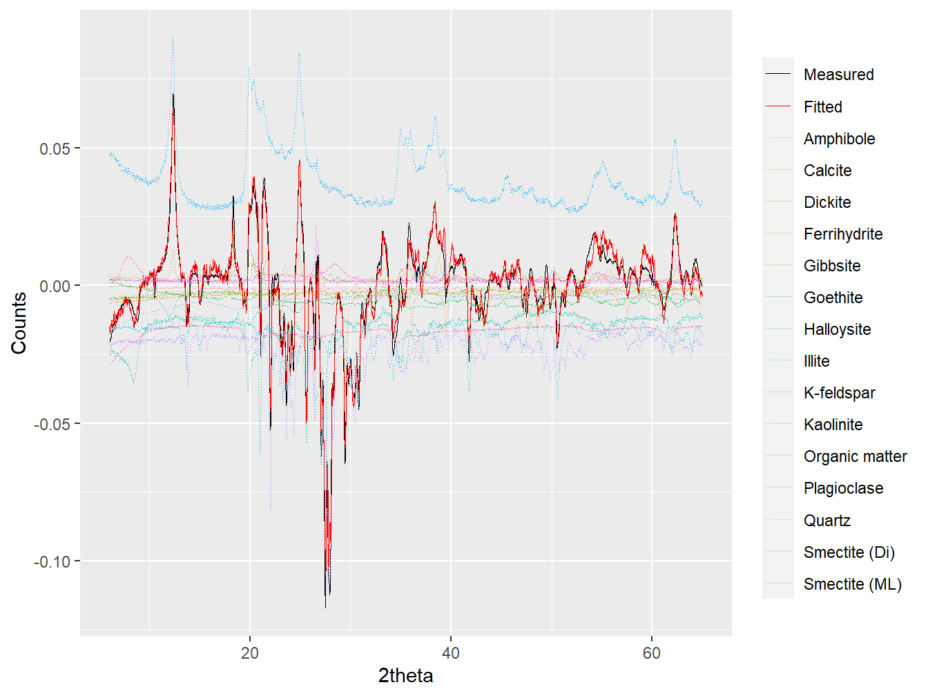
Figure 4.4: Full pattern summation applied to the loading of Dim.2.
dim2_fit$phases_grouped[order(dim2_fit$phases_grouped$coefficient),]## phase_name coefficient
## 12 Plagioclase -1.209673e-03
## 9 K-feldspar -9.533729e-04
## 2 Calcite -4.138665e-04
## 8 Illite -3.952620e-04
## 15 Smectite (ML) -3.182366e-04
## 7 Halloysite -1.450224e-04
## 11 Organic matter -7.906963e-05
## 4 Ferrihydrite -5.087144e-05
## 1 Amphibole -3.251187e-05
## 13 Quartz 1.990181e-05
## 6 Goethite 4.349864e-05
## 14 Smectite (Di) 1.256807e-04
## 3 Dickite 1.287611e-04
## 5 Gibbsite 1.935992e-04
## 10 Kaolinite 9.066849e-04with more negative scores associated with increased plagioclase and K-feldspar peak intensities, and more positive scores associated with increased kaolinite and gibbsite peak intensities. Dim.2 can therefore be interpreted to represent an index of chemical alteration, with higher values representing a greater degree of alteration (i.e. the weathering of feldspars to kaolinite and gibbsite and associated loss of base cations). The same analysis can be applied for the interpretation of subsequent PCA dimensions, but can become increasingly challenging when the loading vector becomes comprised of minor or diffuse features of the XRPD data.
4.3 Fuzzy clustering
Cluster analysis will be now applied to the 5 PCs plotted in Figure 4.1 using fuzzy-c-means clustering algorithm implemented in the e1071 package (Meyer et al. 2021).
When applying cluster analysis, the selection of the most appropriate number of clusters can prove to be subjective and, in some cases, difficult. There are a number of approaches that can be used to objectively define the most appropriate number of clusters (Rossel et al. 2016; Butler et al. 2020), but for simplicity the number of clusters used in this example will be manually defined as 9:
#Apply the fuzzy-c-means algorithm to the PCs
fcm <- cmeans(pca$coords[-1],
              center = 9)

#check the data are in the same order
identical(names(fcm$cluster), pca$coords$sample_id)
## [1] TRUE#Join the data together
clusters <- data.frame("SSN" = names(fcm$cluster),
"CLUSTER" = paste0("C", unname(fcm$cluster)),
pca$coords[-1])
#Reorder the clusters based on Dim.1
#Lowest mean Dim.1 will be Cluster 1
#Highest mean Dim.1 will be Cluster 9
dim1_mean <- aggregate(Dim.1 ~ CLUSTER,
data = clusters,
FUN = mean)
#Order so that the Dim.1 mean is ascending
dim1_mean <- dim1_mean[order(dim1_mean$Dim.1),]
dim1_mean$NEW_CLUSTER <- paste0("C", 1:nrow(dim1_mean))
#Create a named vector that will be used to revalue cluster names
#Values of the vector are the new values, and old values are the names
rv <- setNames(dim1_mean$NEW_CLUSTER, # the vector values
dim1_mean$CLUSTER) #the vector names
#use the revalue function to create a new cluster column
clusters$NEW_CLUSTER <- revalue(clusters$CLUSTER,
rv)
#Create an empty list
p <- list()
#Populate each item in the list using the dimension already
#defined in x and y above
for (i in 1:length(x)) {
p[[i]] <- ggplot(data = clusters) +
geom_point(aes_string(x = paste0("Dim.", x[i]),
y = paste0("Dim.", y[i]),
fill = "NEW_CLUSTER"),
shape = 21,
size = 3,
alpha = 0.5) +
guides(fill = guide_legend(title="Cluster"))
}
grid.arrange(grobs = p,
ncol = 2)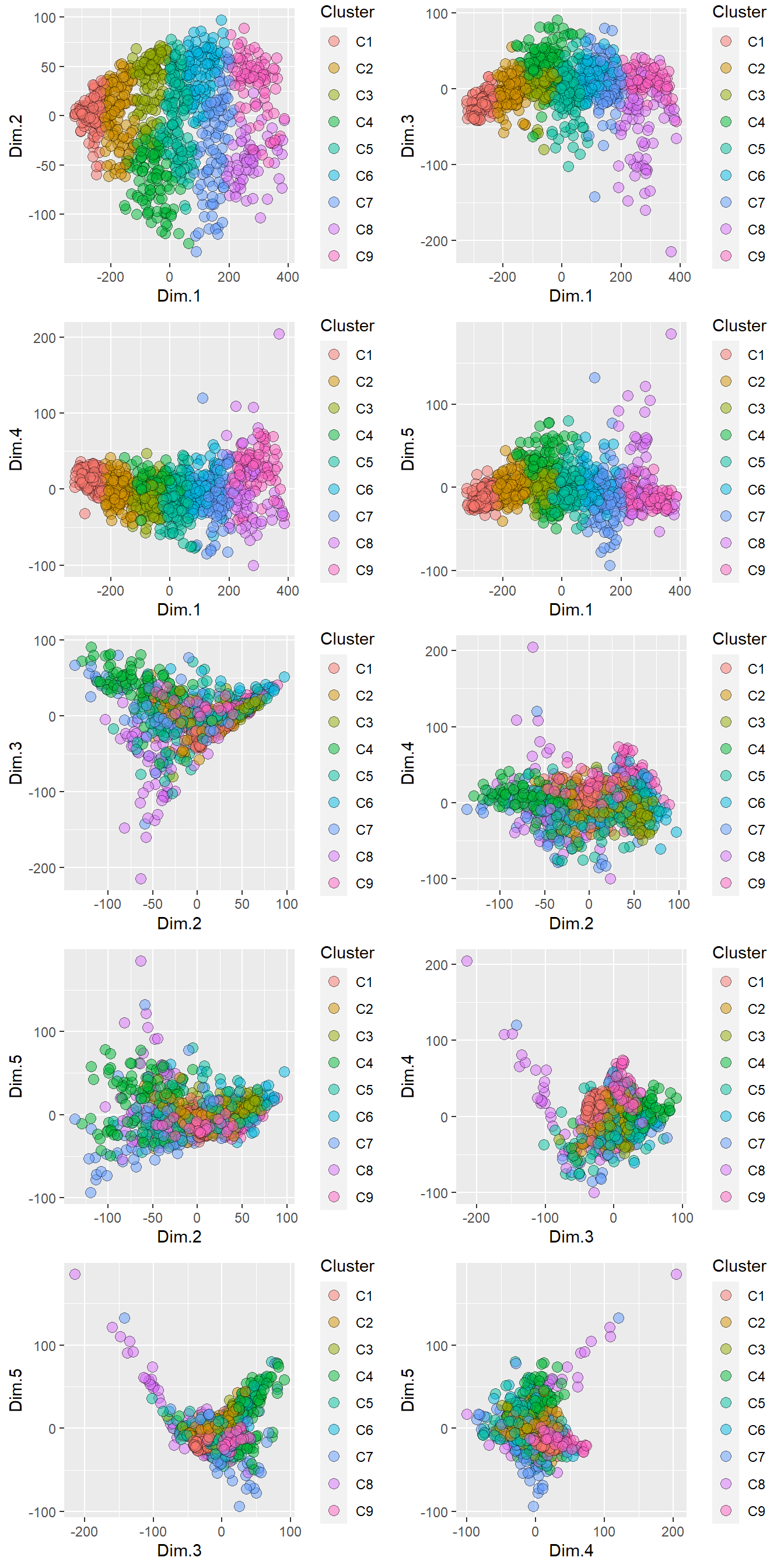
Figure 4.5: Pre-treated XRPD data clustered into 9 groups.
4.3.1 Cluster membership
Use of the fuzzy-c-means clustering algorithm results in every sample having a membership coefficient for each cluster. These membership coefficients range from 0 to 1, with 1 being the highest degree of membership. Below these membership coefficients will be plotted using the first 2 PCs in order to help visualise the ‘fuzzy’ nature of the clustering:
#Extract the membership coefficients
members <- data.frame(fcm$membership, check.names = FALSE)

#Add C to all the names to match that used above.
names(members) <- paste0("C", names(members))

#revalue the names based on the new clustering order
names(members) <- revalue(names(members), rv)

#Add membership to the name
names(members) <- paste0("Membership_", names(members))

#Join clusters and members
members <- data.frame(clusters,
                      members)

#Create and empty list for the plots
p <- list()

#Populate each item in the list using the dimension defined
#in x and y
for (i in 1:9) {

   p[[i]] <- ggplot(data = members) +
             geom_point(aes_string(x = "Dim.1",
                                   y = "Dim.2",
                                   fill = paste0("Membership_C",
                                                 i)),
                        shape = 21,
                        size = 3,
                        alpha = 0.5) +
             ggtitle(paste("Cluster", i)) +
             theme(legend.position = "None") +
             scale_fill_gradient(low = "blue",
                                 high = "red")

}

grid.arrange(grobs = p,
             ncol = 3)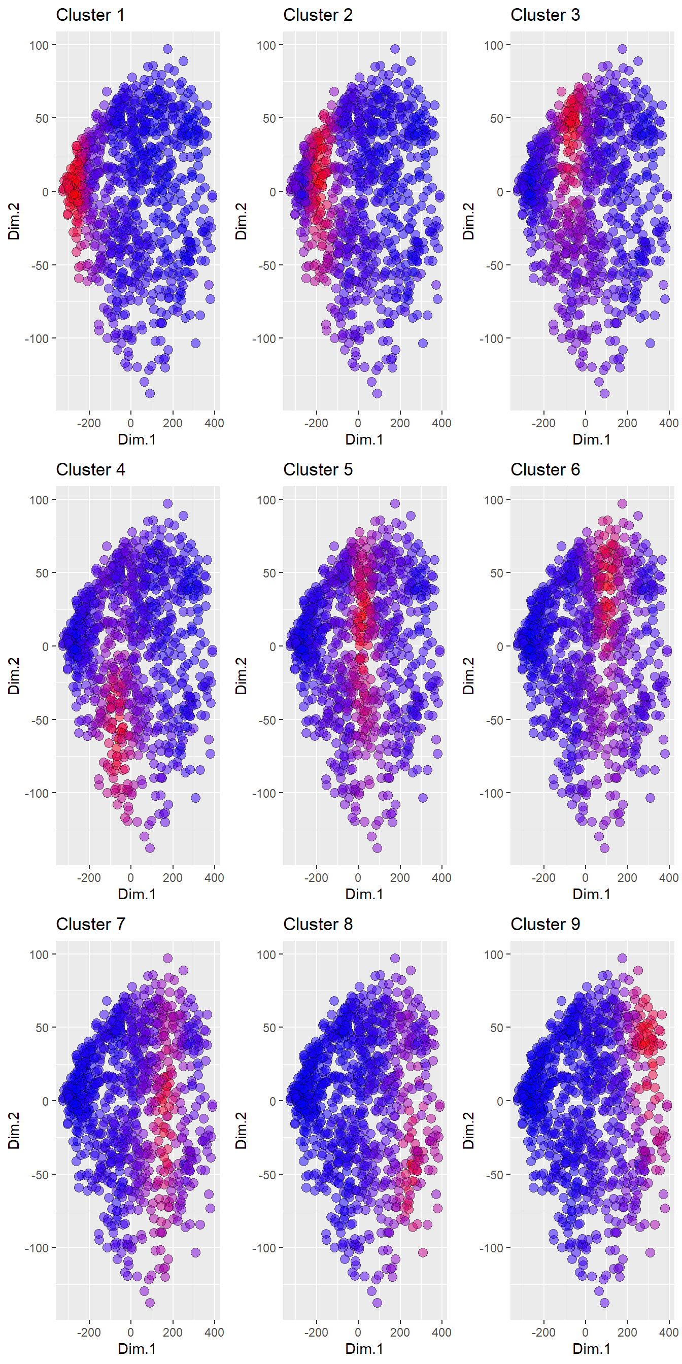
Figure 4.6: Membership coefficients for the nine clusters plotted for the first two PCs. Blue symbols have low membership (~0), whilst red symbols have high membership (~1).
Together Figures 4.5 and 4.6 illustrate how the soil XRPD data in this data set reflect the soil mineralogy continuum, and as such can be challenging to cluster into a discrete number of groups. In particular the membership coefficients in Figure 4.6 help highlight how soils can exist on the boundary of two or more clusters and therefore have similar membership coefficients to numerous clusters. This property is characteristic of most large soil data sets, and can make it challenging to define very distinct clusters. However, the membership coefficients data can be used so that only samples with the highest coefficients are retained, resulting in more distinct mineralogical groups that do no overlap.
4.3.2 Subsetting Clusters
Here, more mineralogically distinct clusters will be created by only retaining samples within each cluster that have a membership coefficient exceeding the 75th percentile:
#Create a blank name to populate with the unique SSNs
member_ssn <- list()

#A loop to omit samples from each cluster with low membership coefficient
for (i in 1:9) {

  memberships <- members[which(members$NEW_CLUSTER == paste0("C", i)),
                         c("SSN", paste0("Membership_C", i))]


  #Extract the samples with top 25 % of membership coefficient for each cluster
  memberships_75 <- which(memberships[[2]] > quantile(memberships[[2]],
                                                      probs = 0.75))

  member_ssn[[i]] <- memberships$SSN[memberships_75]

  names(member_ssn)[i] <- paste0("C", i)

}

#Unlist the indexes
member_ssn <- unname(unlist(member_ssn))

members_sub <- members[which(members$SSN %in% member_ssn),]

#Plot the results
#Create and empty list
p <- list()

#Populate each item in the list using the dimension defined
#in x and y
for (i in 1:length(x)) {

   p[[i]] <- ggplot(data = members_sub) +
             geom_point(aes_string(x = paste0("Dim.", x[i]),
                                   y = paste0("Dim.", y[i]),
                                   fill = "NEW_CLUSTER"),
                        shape = 21,
                        size = 3,
                        alpha = 0.5) +
             guides(fill = guide_legend(title="Cluster"))

}

grid.arrange(grobs = p,
             ncol = 2)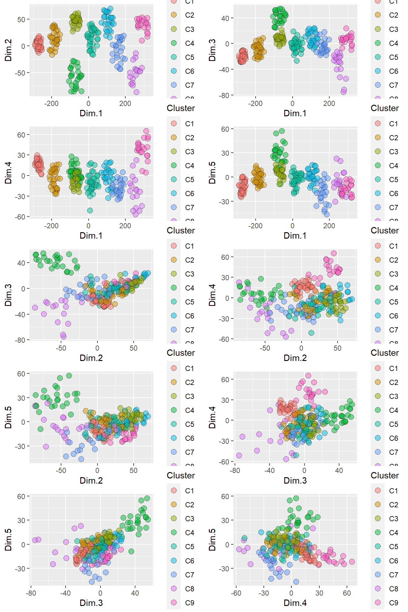
Figure 4.7: The formation of distinct clusters by retaining the samples within each cluster that have membership coefficients greater than the 75% percentile.
4.4 Exploring results
Now that a set of mineralogically distinct clusters have been defined from the data, there are a number of ways that the data can be explored in order to relate the soil mineral composition to the nutrient concentrations. Firstly, since these data are geo-referenced, the spatial distribution of each cluster can be visualised, for example:
clust_sub <- join(members_sub[c("SSN", "NEW_CLUSTER")],
                  props, by = "SSN")

#Plot cluster 9
leaflet(clust_sub[which(clust_sub$NEW_CLUSTER == "C1"), ]) %>%
  addTiles() %>%
  addCircleMarkers(~Longitude, ~Latitude)
Figure 4.8: Interactive map of the soil samples associated with Cluster 9.
returns a map of the locations of all samples within Cluster 9. Even though samples within this cluster are dispersed across sub-Saharan Africa, their XRPD signals (and, hence mineralogies) are very similar, which can readily be plotted with a little manipulation of the data:
#Create a blank list to populate
cluster_xrpd <- list()

for (i in 1:9) {
cluster_xrpd[[i]] <- xrpd_aligned[clust_sub$SSN[clust_sub$NEW_CLUSTER == paste0("C",i)]]
names(cluster_xrpd)[i] <- paste0("C", i)
}

#Plot cluster 9
plot(as_multi_xy(cluster_xrpd$C1), wavelength = "Cu", normalise = TRUE)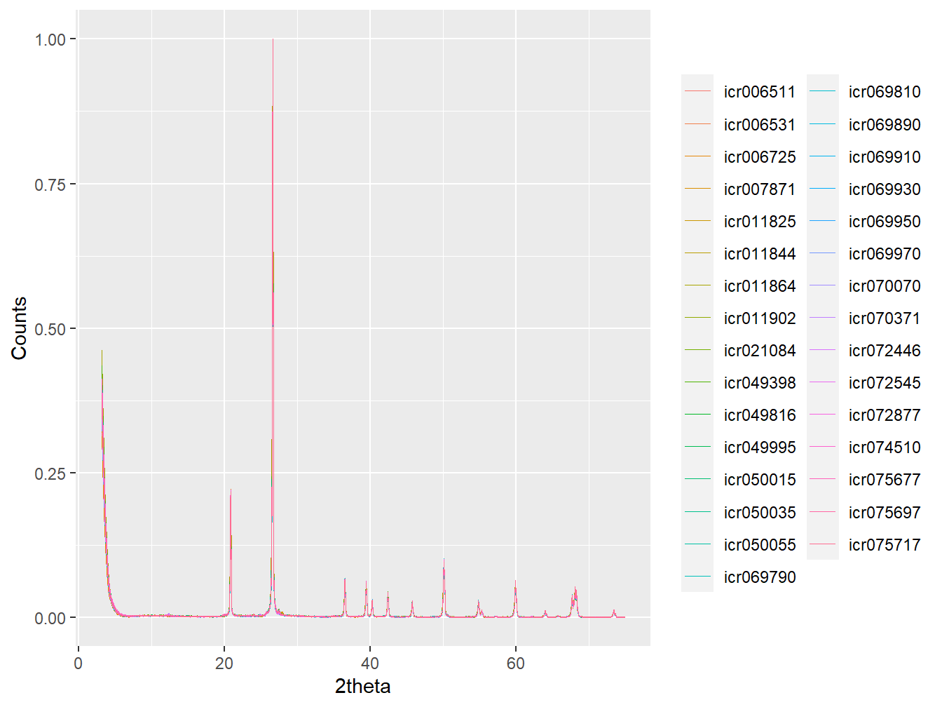
Figure 4.9: Clustered pre-treated XRPD from Cluster 9.
Given that the soil mineral composition ultimately governs the total concentrations of nutrients and their phyto-availability, the nine mineralogically different clusters defined here should display contrasting geochemical properties. These geochemical properties are present in the props data that has already been combined with the clustering data in clust_sub. Here the relative enrichments and deficiencies of each cluster with respect to total nutrient concentrations will be visualised using barplots (Montero-Serrano et al. 2010; Butler et al. 2020):
#Select the variables of interest
total_nutrients <- subset(clust_sub,
                          select = c(NEW_CLUSTER,
                                     TOC, K, Ca,
                                     Mn, Fe, Ni,
                                     Cu, Zn))

#Create geometric mean function
gmean <- function(x) {exp(mean(log(x)))}

#Compute overall geometric means for each nutrient (i.e. column)
total_nutrients_gmeans <- apply(total_nutrients[-1], 2, gmean)

#Compute the geometric mean for each nutrient by cluster
cluster_gmeans <- by(total_nutrients[-1],
                     as.factor(total_nutrients$NEW_CLUSTER),
                     function(x) apply(x, 2, gmean))

#Bind the data by row
cluster_gmeans <- do.call(rbind, cluster_gmeans)

#Calculate log-ratios by dividing by the geometric mean
#of each nutrient
bp <- apply(cluster_gmeans,1,
            function(x) log(x/total_nutrients_gmeans))


#Use melt from the reshape2 package so that the data are
#in the right format for ggplot2:
bpm <- melt(bp)

#Create a barplot using ggplot2
g1 <- ggplot(bpm,
             aes(fill=Var1, y=value, x=Var2)) +
      geom_bar(position="dodge", stat="identity") +
      theme(legend.title = element_blank()) +
      xlab("Cluster") +
      ylab("")

#Make the barplot interactive
ggplotly(g1)
Figure 4.10: Average total nutrient concentrations of each cluster expressed as deviation in log-ratio scale from the geometric mean. Values below zero represent average concentrations lower than that for the entire dataset, whilst values above zero represent the opposite.
The resulting barplot illustrates how the nine clusters defined by the XRPD data are characterised by contrasting geochemical compositions. Clusters 8 and 9 are by far the most deficient in all nutrients, whilst Clusters 1, 2 and 3 are enriched in all nutrients (with the exception of K in Cluster 1). Interestingly, soils in Cluster 6 have the highest concentrations of total K on average, but are generally deficient in other nutrients. The relationships between the geochemical compositions of each cluster and the mineralogy can be interpreted by quantifying the mean diffractogram of each cluster using the full pattern summation functions outlined in Chapter 2:
#Create a blank list to be populated
xrpd_clusters <- list()

#Calculate the mean diffractogram of each cluster
for (i in 1:9) {

  #Extract the SSN for the cluster
  ssns <- clust_sub$SSN[which(clust_sub$NEW_CLUSTER == paste0("C", i))]

  #Extract the aligned xrpd data and make sure it is a multiXY object
  xrpd_clusters[[i]] <- as_multi_xy(xrpd_aligned[ssns])

  names(xrpd_clusters)[i] <- paste0("C", i)

  #Convert to a data frame
  xrpd_clusters[[i]] <- multi_xy_to_df(xrpd_clusters[[i]],
                                       tth = TRUE)

  #Calculate mean diffractogram
  xrpd_clusters[[i]] <- as_xy(data.frame("tth" = xrpd_clusters[[i]]$tth,
                                         "counts" = rowMeans(xrpd_clusters[[i]][-1])))

}

#Plot the mean diffractogram of Cluster 9
plot(xrpd_clusters$C1, wavelength = "Cu")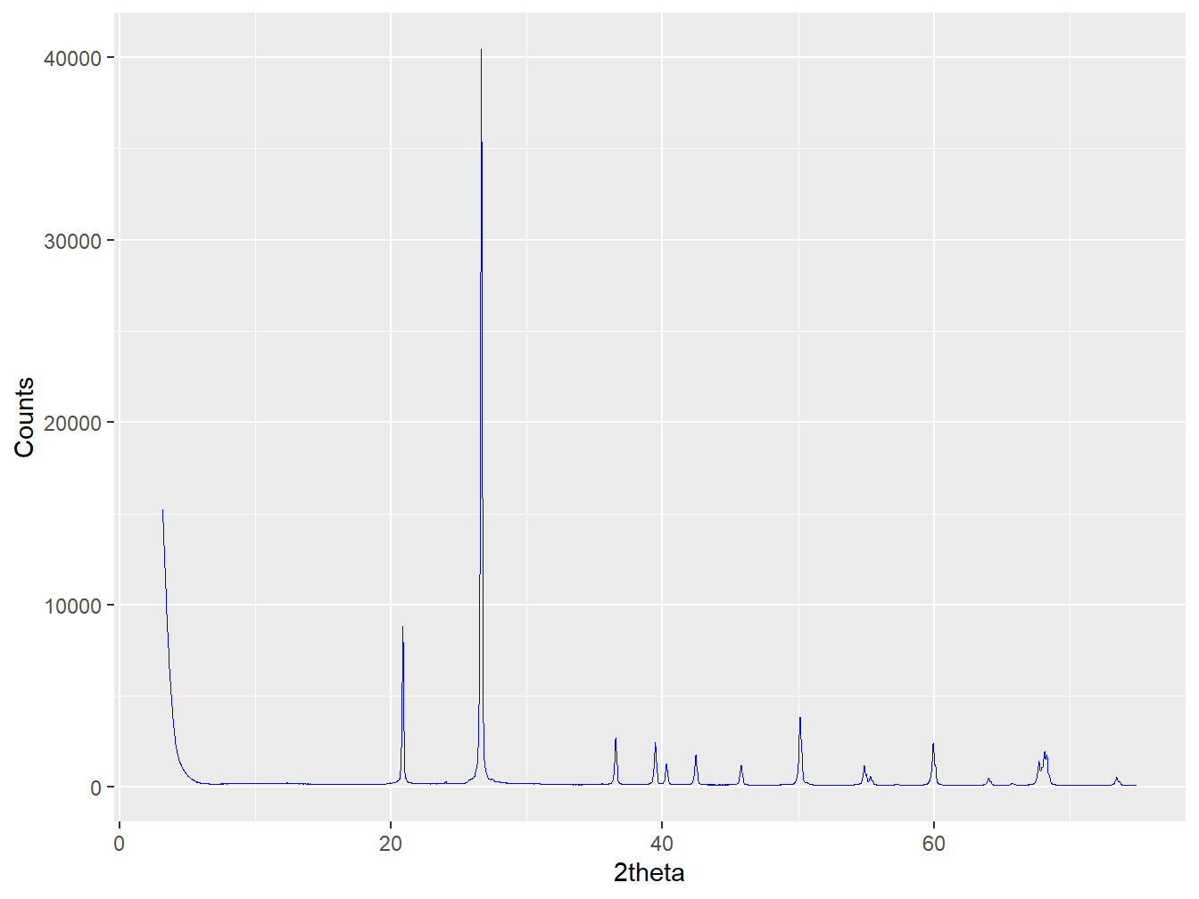
Figure 4.11: The mean diffractogram of Cluster 9.
Now that the mean diffractogram of each cluster has been computed. The mineralogy of each diffractogram can be quantified using afps() using therockjock_afsis library created above, yielding an approximate average of the mineral composition of each cluster:
#Define the names of the minerals to supply to afps
usuals <- c("Quartz", "Kaolinite",
            "Halloysite", "Dickite",
            "Smectite (Di)", "Smectite (ML)",
            "Illite", "Mica (Di)", "Muscovite",
            "K-feldspar", "Plagioclase",
            "Goethite", "Maghemite", "Ilmenite",
            "Hematite", "Gibbsite", "Magnetite",
            "Anatase", "Amphibole", "Pyroxene",
            "Calcite", "Gypsum", "Organic matter",
            "HUMIC_ACID", "FERRIHYDRITE_HUMBUG_CREEK",
            "FERRIHYDRITE",
            "BACK_POS")

#Define the amorphous phases
amorph <- c("ORGANIC_MATTER", "ORGANIC_AFSIS",
            "HUMIC_ACID", "FERRIHYDRITE_HUMBUG_CREEK",
            "FERRIHYDRITE")

clusters_quant <- lapply(xrpd_clusters, afps,
                         lib = rockjock_afsis,
                         std = "QUARTZ_1_AFSIS",
                         refs = usuals,
                         amorphous = amorph,
                         align = 0.2,
                         lod = 0.05,
                         amorphous_lod = 0,
                         force = "BACK_POS")

#Load the regrouping structures for rockjock and afsis
data(rockjock_regroup)
data(afsis_regroup)

#lapply the regrouping structure
clusters_quant_rg <- lapply(clusters_quant,
                            regroup,
                            y = rbind(rockjock_regroup[1:2],
                                      afsis_regroup[1:2]))

#Extract the quantitative data
quant_table <- summarise_mineralogy(clusters_quant_rg,
                                    type = "grouped",
                                    order = TRUE)

#Reduce to the 10 most common phases for a barplot
quant_table <- quant_table[2:11]
The resulting quantification can then be plotted:
#Rename clusters C1 to C9
rownames(quant_table) <- paste0("C", rownames(quant_table))

#Use melt from the reshape2 package so that the data are
#in the right format for ggplot2:
quant_table_m <- melt(as.matrix(quant_table))

#Create a barplot using ggplot2
g2 <- ggplot(quant_table_m,
             aes(fill=Var2, y=value, x=Var1)) +
      geom_bar(position="dodge", stat="identity") +
      theme(legend.title = element_blank()) +
      xlab("Cluster") +
      ylab("")

#Make the barplot interactive
ggplotly(g2)
Figure 4.12: Mineral compositions of the nine clusters based on the mean diffractogram
Together the geochemical (Figure 4.10) and mineralogical (Figure 4.12) barplots can be used to interpret a range of relationships between the soil mineral composition and the nutrient concentrations, for instance:
- The notable K enrichment in the soils of Cluster 6 most likely results from the relatively high concentrations of K-feldspar minerals in these soils.
- Soils in Clusters 8 and 9 are deficient in all nutrients due to the dominance of quartz in combination with a near absence of clay minerals and/or Fe/Ti(hydr)oxides
- Soils in Cluster 2 are particularly enriched in Ca due to the high concentrations of plagioclase, expandable/ML clays and calcite (not plotted but can be observed in the tabulated data) minerals.
This example ultimately acts to highlight the utility of ‘Digital’ methods of analysis applied to soil XRPD data. Whilst this example focuses on total nutrient concentrations, the method can also be applied to the Mehlich-3 extractable element concentrations that are also included within the props data. For further analysis and discussion on the application of cluster analysis to this dataset, along with additional methods of compositional data analysis, see Butler et al. (2020) and the accompanying Supplementary Material.