Chapter 1 Working with XRPD data in R
At this stage it is assumed that you have R and RStudio installed on your computer and have installed the powdR package using install.packages("powdR"). For brief introductions to R, the RStudio website has links to useful material. One aspect worth noting is that any R function used throughout this document will have additional help associated with it that can be accessed using ?. For example, to access help on the mean() function, use ?mean.
This chapter will work through:
1.1 The basic form of XRPD data
In its most basic form, XRPD (X-ray powder diffraction) data (often referred to as a diffractogram) is simply comprised of an x-axis (in units of 2θ) and y-axis (counts at the 2θ positions). The following figure shows a diffratogram for a soil from north east Scotland.
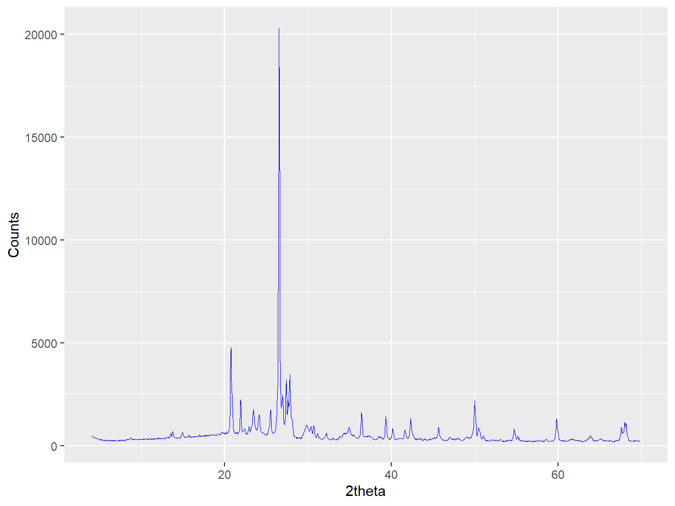
Figure 1.1: A diffractogram of a soil developed from Granite in north east Scotland
Each mineral contributing to the observed diffractogram contributes peaks at specific locations along the x-axis, each with characteristic relative intensities to one-another that are defined by the crystal structure and chemistry. Each mineral can therefore be considered to have a unique signature. For quartz, an omnipresent mineral in the world’s soils, this signature is relatively simple:
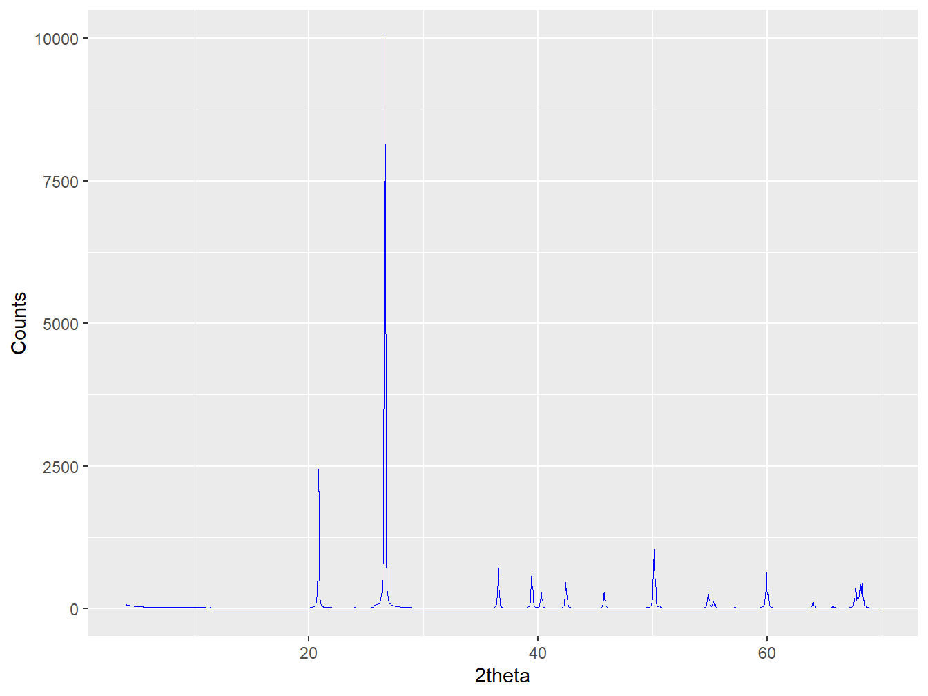
Figure 1.2: A diffractogram of quartz
whereas other soil minerals such as K-feldspar have very different peak positions and relative intensities that again are governed by the mineral’s crystal structure and chemistry:
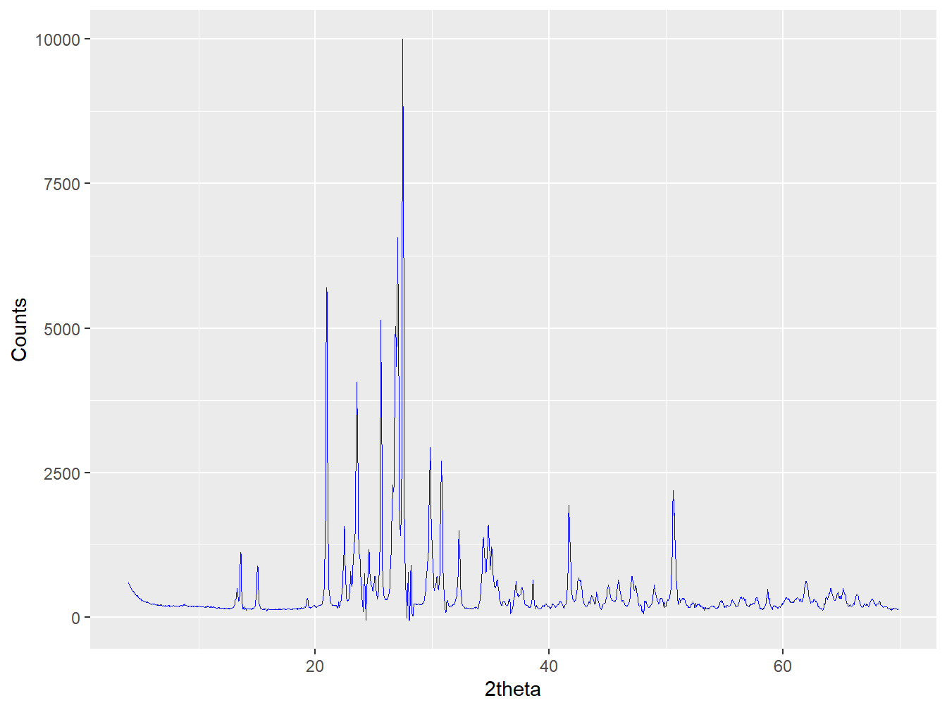
Figure 1.3: A diffractogram of K-feldspar (orthoclase)
In any given diffractogram of a material like a soil there can be multiple minerals contributing their unique signature to the observed pattern, which ends up simply being the weighted sum of these signatures. The proportion of each minerals pattern in the mixture is inherently related to a given minerals concentration within the mixture but to extract that we also need to know some scaling factors based on the defined ‘diffracting power’ of each mineral, known as Reference Intensity Ratios (see Chapter 2). Together these principles make XRPD the most widely used analytical technique for qualitative (what minerals are present?) and quantitative (how much of each mineral?) soil mineralogy.
1.2 Loading XRPD data
In order to work with XRPD data in R, it first needs to be loaded. XRPD data come in all sorts of proprietary formats (e.g. .raw, .dat and .xrdml), which can make this initial stage of loading data more complicated than it needs to be. As described above, XRPD data is most simply comprised of an x-axis (2θ) and y-axis (counts), and all XRPD data loaded into R throughout this documentation will hence take this XY form. Here 2 options for loading proprietary XRPD data into R will be described.
1.2.1 Option 1: PowDLL
The free software PowDLL written by Nikoloas Kourkoumelis, offers excellent functionality for the conversion of different XRPD file types. PowDLL can import and export a large range of XRPD file types including ‘.xy’ files that can readily be loaded into R or any text editor. These ‘.xy’ files are an ASCII format that simply comprises the two variables (2θ and counts) separated by a space. The following video from Phys Whiz on YouTube illustrates use of powDLL to create the ‘.xy’ files that we seek to use.
Once you have your ‘.xy’ files, they can be loaded into R using the read_xy() function from the powdR package. The following reproducible example uses files that are stored within powdR and were recorded on a Siemens D5000 using Co-K\(\alpha\) radiation.
#load the powdR package
library(powdR)

#Extract the path of the file from the powdR package
file <- system.file("extdata/D5000/xy/D5000_1.xy", package = "powdR")

#Load the file as an object called xy1
xy1 <- read_xy(file)
#Explore the xy data
summary(xy1)## tth counts
## Min. : 2.00 Min. : 70.0
## 1st Qu.:20.25 1st Qu.: 145.0
## Median :38.50 Median : 236.0
## Mean :38.50 Mean : 292.9
## 3rd Qu.:56.75 3rd Qu.: 342.0
## Max. :75.00 Max. :6532.0#check the class of xy data
class(xy1)## [1] "XY" "data.frame"Notice how the class of xy1 is both XY and data.frame. This means that various additional methods for each of these types of object classes can be used to explore and analyse the data. These methods can be viewed using:
methods(class = "XY")## [1] align_xy interpolate plot
## see '?methods' for accessing help and source codewhich shows how functions align_xy(), interpolate() and plot() all have methods for XY class objects. Help on each of these can be sourced using ?align_xy.XY, ?interpolate.XY and ?plot.XY, respectively. When calling these functions it is not necessary to specify the .XY suffix because R will recognise the class and call the relevant method.
1.2.2 Option 2: Loading directly into R
Alternatively to PowDLL, the extract_xy() function in the powdR package can extract the XY data from a wide range of proprietary XRPD file formats straight into R via the xylib C++ library implemented behind the scenes in the rxylib package (Kreutzer and Johannes Friedrich 2020).
#Extract the path of the file from the powdR package
file <- system.file("extdata/D5000/RAW/D5000_1.RAW", package = "powdR")

#Load the file as an object called xy2
xy2 <- extract_xy(file)
##
## [read_xyData()] >> File of type Siemens/Bruker RAW detected#Summarise the xy data
summary(xy2)## tth counts
## Min. : 2.00 Min. : 70.0
## 1st Qu.:20.25 1st Qu.: 145.0
## Median :38.50 Median : 236.0
## Mean :38.50 Mean : 292.9
## 3rd Qu.:56.75 3rd Qu.: 342.0
## Max. :75.00 Max. :6532.0#Check the class of xy2
class(xy2)## [1] "XY" "data.frame"A word of warning with extract_xy() is that it does not work with all proprietary file types. In particular you may experience problems with Bruker ‘.raw’ files, in which case the use of PowDLL outlined above is recommended instead.
1.2.3 Loading multiple files
The two approaches for loading XRPD data outlined above can also be used to load any number of files into R at once. read_xy() and extract_xy() will recognise cases where more than one file path is supplied and therefore load the files into a multiXY object.
1.2.3.1 read_xy()
There are five ‘.xy’ files stored within a directory of the powdR package that can be loaded into a multiXY object via:
paths1 <- dir(system.file("extdata/D5000/xy", package = "powdR"),
full.names = TRUE)
#Now read all files in the directory
xy_list1 <- read_xy(paths1)
#Check the class of xy_list1
class(xy_list1)## [1] "multiXY" "list"The resulting multiXY object is a list of XY objects, with each XY object being a data frame comprised of the 2θ and count intensities of the XRPD data.
#Check the class of each item within the multiXY object
lapply(xy_list1, class)## $D5000_1
## [1] "XY" "data.frame"
##
## $D5000_2
## [1] "XY" "data.frame"
##
## $D5000_3
## [1] "XY" "data.frame"
##
## $D5000_4
## [1] "XY" "data.frame"
##
## $D5000_5
## [1] "XY" "data.frame"Each sample within the list can be accessed using the $ symbol. For example:
#Summarise the data within the first sample:
summary(xy_list1$D5000_1)## tth counts
## Min. : 2.00 Min. : 70.0
## 1st Qu.:20.25 1st Qu.: 145.0
## Median :38.50 Median : 236.0
## Mean :38.50 Mean : 292.9
## 3rd Qu.:56.75 3rd Qu.: 342.0
## Max. :75.00 Max. :6532.0Alternatively, the same item within xy_list1 could be accessed using xy_list1[[1]]. In the same way the XY class objects have methods associated with them, there are a number of different methods for multiXY objects:
methods(class = "multiXY")## [1] align_xy interpolate multi_xy_to_df plot
## see '?methods' for accessing help and source codewhich include align_xy(), interpolate(), multi_xy_to_df() and plot that are all detailed in subsequent sections.
1.2.3.2 extract_xy()
In addition to the five ‘.xy’ files loaded above, there are also five ‘.RAW’ files stored within a separate directory of powdR, which can be loaded in a similar fashion using extract_xy():
paths2 <- dir(system.file("extdata/D5000/RAW", package = "powdR"),
full.names = TRUE)
#Now read all files in the directory
xy_list2 <- extract_xy(paths2)##
## [read_xyData()] >> File of type Siemens/Bruker RAW detected
##
## [read_xyData()] >> File of type Siemens/Bruker RAW detected
##
## [read_xyData()] >> File of type Siemens/Bruker RAW detected
##
## [read_xyData()] >> File of type Siemens/Bruker RAW detected
##
## [read_xyData()] >> File of type Siemens/Bruker RAW detected#Find out what the xy_list2 is
class(xy_list2)## [1] "multiXY" "list"which yields xy_list2 that is identical to xy_list1:
all.equal(xy_list1, xy_list2)## [1] TRUE1.3 Plotting XRPD data
The powdR package contains plot() methods for both XY and multiXY objects (see ?plot.XY and ?plot.multiXY).
1.3.1 Plotting XY objects
An XY object can be plotted by:
plot(xy1, wavelength = "Co", interactive = FALSE)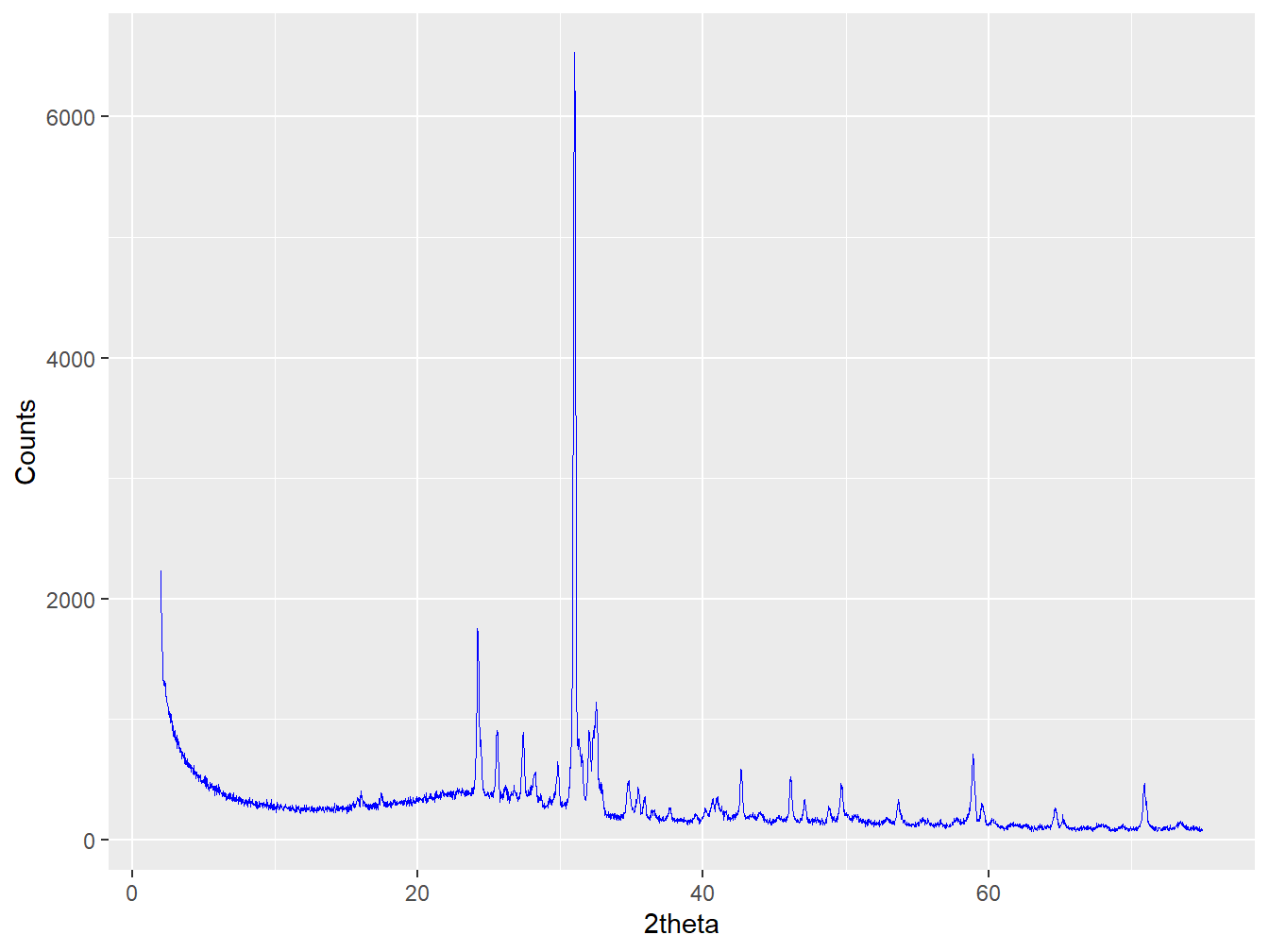
Figure 1.4: An example figure created using the plot method for an XY object.
where wavelength = "Co" is required so that d-spacings can be computed and displayed when interactive = TRUE.
1.3.2 Plotting multiXY objects
Often it’s useful to plot more than one pattern at the same time, which can be achieved by plotting a multiXY object:
plot(xy_list1, wavelength = "Co", interactive = FALSE)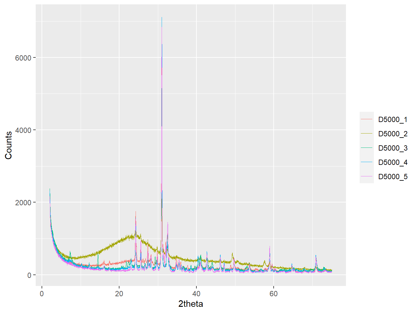
Figure 1.5: An example figure created using the plot method for a multiXY object.
As above, using interactive = TRUE in the function call will instead produce an interactive plot. In addition, the plotting of XY and multiXY objects also allows you to alter the x-axis limits and normalise the count intensities for easier comparison of specific peaks:
plot(xy_list1, wavelength = "Co",
     xlim = c(30, 32), normalise = TRUE)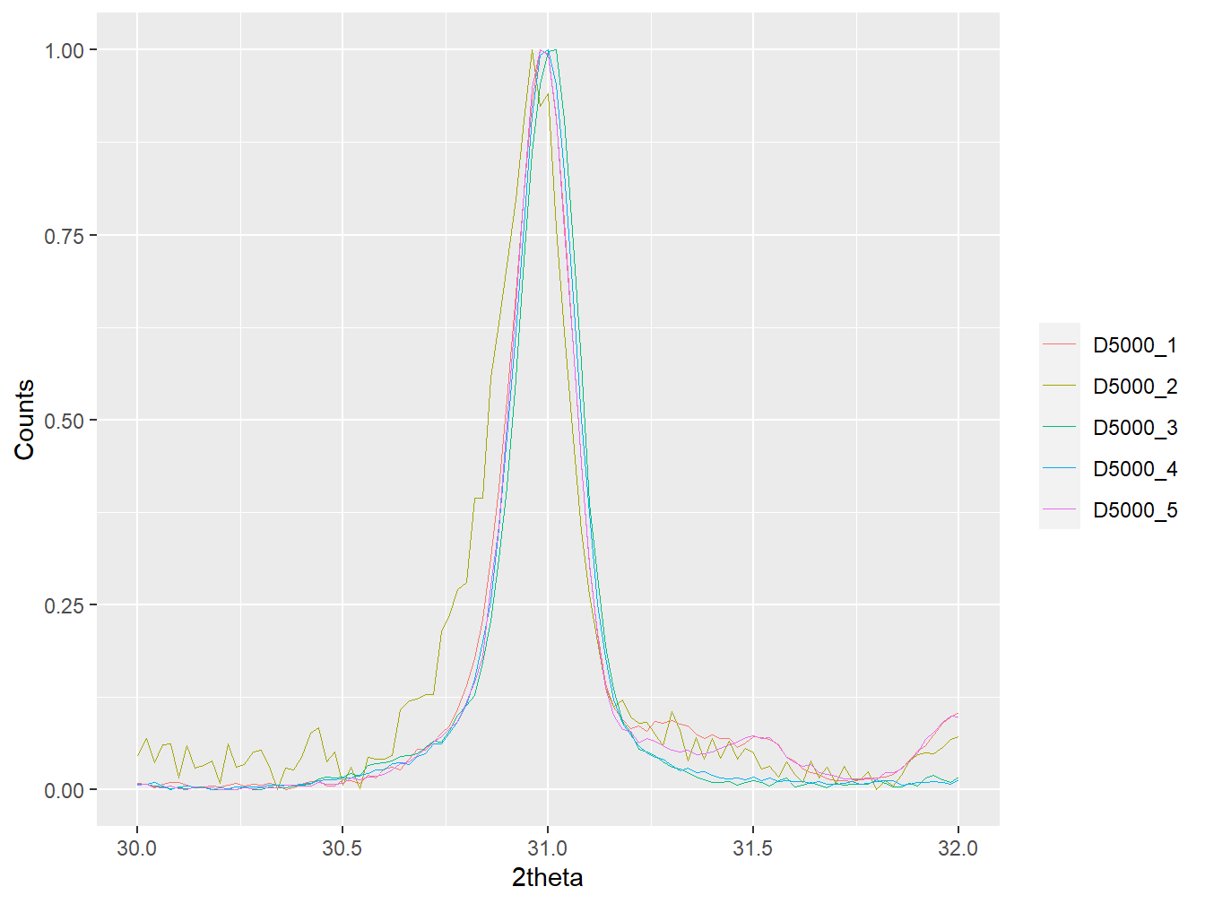
Figure 1.6: An example figure created using the plot method for an XY object with normalised count intensities and a restrict x-axis.
1.3.3 Modifying plots with ggplot2
All plots shown so far are produced behind the scenes using the ggplot2 package, which will already be present on your machine if you have installed powdR. This means that it is possible to modify the plots in different ways by adding subsequent ggplot2 layers, each separated by +. For example, it’s possible to add points of the quartz peak intensities extracted from a crystal structure database using geom_point(), and then add a title using ggtitle(), followed by changing the theme using theme_bw().
#Define the relative intensities of quartz peaks
quartz <- data.frame("tth" = c(24.22, 30.99, 42.61, 46.12,
                               47.06, 49.62, 53.62, 58.86,
                               64.60, 65.18, 70.79, 73.68),
                     "intensity" = c(0.20, 1.00, 0.06, 0.06,
                                     0.03, 0.05, 0.03, 0.11,
                                     0.03, 0.01, 0.07, 0.03))

#Load the ggplot2 package
library(ggplot2)

#Create a plot called p1
p1 <- plot(xy1, wav = "Co", normalise = TRUE) +
           geom_point(data = quartz, aes(x = tth, y = intensity), size = 5,
             shape = 21, colour = "red") +
           ggtitle("A soil with quartz peaks identified") +
           theme_bw()

p1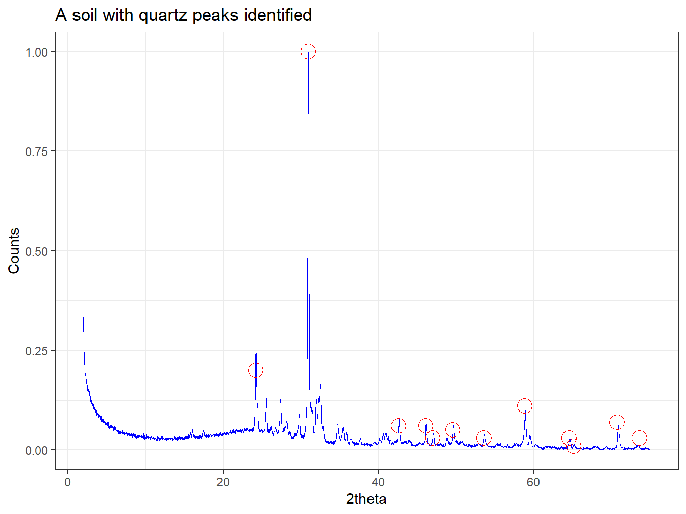
Figure 1.7: A quartz diffractogram with the locations and relative intensities of the quartz peaks identified.
Further help on using the ggplot2 package to build up plots in layers is provided in Hadley Wickham’s excellent documentation on data visualization.
Plots produced using ggplot2 are static by default and can be exported as high quality images or pdfs. In some cases it is also useful to produce an interactive plot, which in the case of XRPD data allows for easy inspection of minor features. For most plots creating using ggplot2, the ggplotly() function from the plotly package can be used to convert them into interactive HTML plots that will load either in RStudio or your web browser:
library(plotly)

ggplotly(p1)
1.4 Manipulating XRPD data
Loading XRPD data into R opens up almost limitless capabilities for analysing and manipulating the data via the R language and the thousands of open source packages that enhance its functionality. Here some common forms of XRPD data manipulation will be introduced:
- Subsetting
- Transformations of count intensities
- Interpolation
- Alignment
- Background fitting
- Converting to data frames
- 2θ transformation
1.4.1 Subsetting XRPD data
Quite often the analysis of XRPD data may be applied to a reduced 2θ range compared to that measured on the diffractometer. This can readily be achieved in R for any number of samples.
By summarising xy1 we can see that the 2θ column has a minimum of 2 and a maximum of 75 degrees.
summary(xy1)## tth counts
## Min. : 2.00 Min. : 70.0
## 1st Qu.:20.25 1st Qu.: 145.0
## Median :38.50 Median : 236.0
## Mean :38.50 Mean : 292.9
## 3rd Qu.:56.75 3rd Qu.: 342.0
## Max. :75.00 Max. :6532.0If we wanted to reduce this to the range of 10–60 \(^\circ\) 2θ then we have a couple of options. First we could extract the relevant data directly using the [,] notation for a data frame, where values before the comma represent rows and values after the comma represent columns:
xy1_sub <- xy1[xy1$tth >= 10 & xy1$tth <= 60, ]

summary(xy1_sub)
## tth counts
## Min. :10.0 Min. : 93.0
## 1st Qu.:22.5 1st Qu.: 174.0
## Median :35.0 Median : 256.0
## Mean :35.0 Mean : 308.2
## 3rd Qu.:47.5 3rd Qu.: 345.0
## Max. :60.0 Max. :6532.0This first option is quite simple, but if we wanted to apply it to a list of patterns then using the subset() function would be a far better option.:
xy1_sub2 <- subset(xy1, tth >= 10 & tth <= 60)
identical(xy1_sub, xy1_sub2)## [1] TRUEWhen using a function like subset(), it is very easy to apply it to any number of patterns in a multiXY object or list using lapply():
xy_list1_sub <- lapply(xy_list1, subset,
tth >= 10 & tth <= 60)
#Similarly we can summarise the data in the list again
lapply(xy_list1_sub, summary)## $D5000_1
##       tth           counts
##  Min.   :10.0   Min.   :  93.0
##  1st Qu.:22.5   1st Qu.: 174.0
##  Median :35.0   Median : 256.0
##  Mean   :35.0   Mean   : 308.2
##  3rd Qu.:47.5   3rd Qu.: 345.0
##  Max.   :60.0   Max.   :6532.0
##
## $D5000_2
## tth counts
## Min. :10.0 Min. : 176
## 1st Qu.:22.5 1st Qu.: 361
## Median :35.0 Median : 469
## Mean :35.0 Mean : 557
## 3rd Qu.:47.5 3rd Qu.: 730
## Max. :60.0 Max. :2094
##
## $D5000_3
## tth counts
## Min. :10.0 Min. : 74.0
## 1st Qu.:22.5 1st Qu.: 154.0
## Median :35.0 Median : 193.0
## Mean :35.0 Mean : 240.6
## 3rd Qu.:47.5 3rd Qu.: 251.0
## Max. :60.0 Max. :5150.0
##
## $D5000_4
## tth counts
## Min. :10.0 Min. : 64
## 1st Qu.:22.5 1st Qu.: 133
## Median :35.0 Median : 168
## Mean :35.0 Mean : 223
## 3rd Qu.:47.5 3rd Qu.: 216
## Max. :60.0 Max. :7110
##
## $D5000_5
## tth counts
## Min. :10.0 Min. : 51.0
## 1st Qu.:22.5 1st Qu.: 102.0
## Median :35.0 Median : 133.0
## Mean :35.0 Mean : 202.3
## 3rd Qu.:47.5 3rd Qu.: 183.0
## Max. :60.0 Max. :6837.01.4.2 Transformations of count intensities
As will be introduced in subsequent chapters, log and root transforms of the count intensities of XRPD data can be useful when applying data mining or machine learning methods. By writing a function these transformations can be applied to any number of patterns in just a few lines of code:
#Create a function for log-transforming counts
log_xrpd <- function (x) {

  x[[2]] <- log10(x[[2]])

  return(x)

}

#apply the function to a list of XRPD data
xy_list1_log <- lapply(xy_list1,
                       log_xrpd)

#Plot the transformed data
plot(as_multi_xy(xy_list1_log), wavelength = "Cu")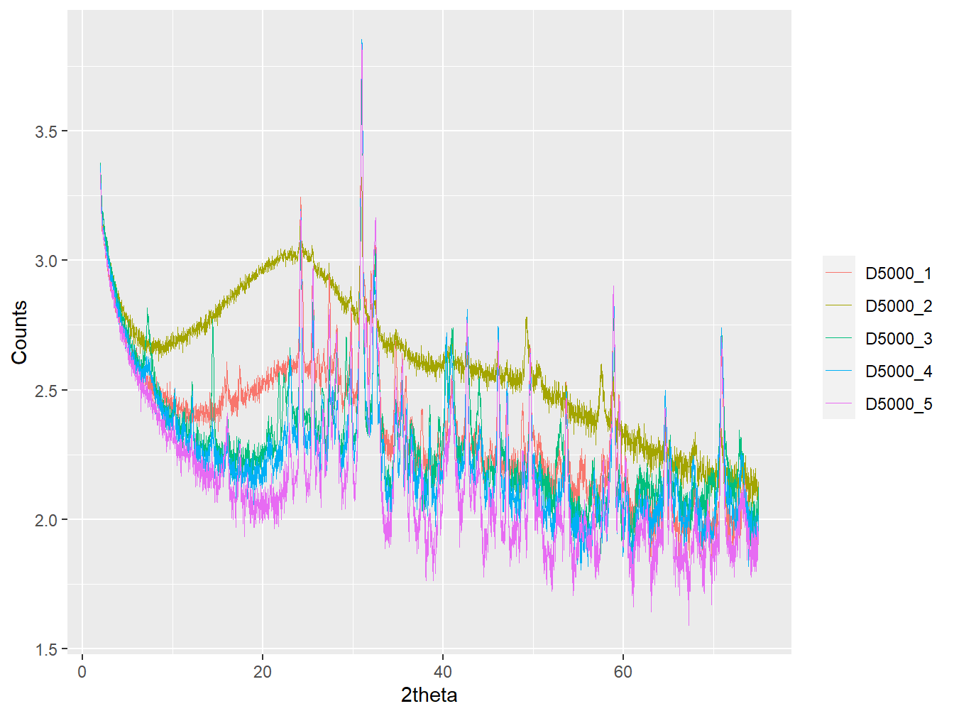
Figure 1.8: Log transformed XRPD data.
Note how the use of x[[2]] in the function represents the second column of x. Alternatively, the form x$counts could be used but the function would fail to run if the variable name was altered in any way.
1.4.3 Interpolation
Sometimes XRPD patterns within a given data set may contain a number of different 2θ axes due to the measurements being carried out on different instruments or on the same instrument but with a different set-up. Direct comparison of such data requires that they are interpolated onto the same 2θ axis.
Here a data set containing 2 samples with different 2θ axes will be created using the soils and rockjock_mixtures data that are pre-loaded within the powdR package:
two_instruments <- as_multi_xy(list("a" = soils$granite,
                                    "b" = rockjock_mixtures$Mix2))

plot(two_instruments, wavelength = "Cu", normalise = TRUE)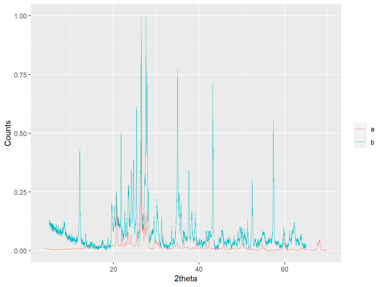
Figure 1.9: Diffractograms from two different instruments.
In this example, the data within the two_instruments list will be interpolated onto an artificial 2θ axis called new_tth, which ranges from 10 to 60 \(^\circ\) 2θ with a resolution of 0.02:
new_tth <- seq(10, 60, 0.02)

two_instruments_int <- interpolate(two_instruments, new_tth)

plot(two_instruments_int, wavelength = "Cu", normalise = TRUE)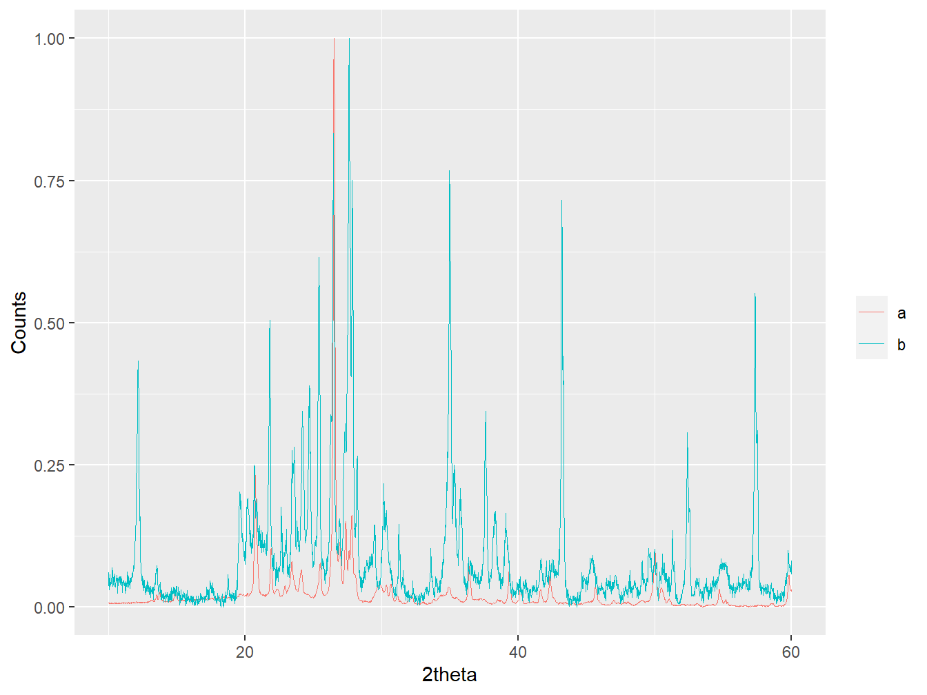
Figure 1.10: Interpolated diffractograms from two different instruments.
1.4.4 Alignment
Peak positions in XRPD data commonly shift in response to small variations in specimen height in the instrument, the so called ‘specimen displacement error’. Even seemingly small misalignments between peaks in different diffractograms can hinder the analysis of XRPD data (Butler et al. 2019). One approach to deal with such peak shifts is to use a mineral with essentially invariant peak positions as an internal standard (e.g. the common mineral quartz), resulting in well aligned data by adding or subtracting a fixed value to the 2θ axis. (Note that the ’specimen displacement error is non linear in 2θ, but a simply linear correction is often satisfactory for most purposes over the typical 2θ range recorded for soil samples)
The powdR package contains functionality for aligning single or multiple patterns using the align_xy() function. In the following examples, samples will be aligned to a pure quartz pattern that will be loaded from the powdR package using read_xy()
#Extract the location of the quartz xy file
quartz_file <- system.file("extdata/minerals/quartz.xy", package = "powdR")

#load the file
quartz <- read_xy(quartz_file)

#Plot the main quartz peak for pure quartz and a sandstone-derived soil
plot(as_multi_xy(list("quartz" = quartz,
                      "sandstone" = soils$sandstone)),
     wavelength = "Cu",
     normalise = TRUE,
     xlim = c(26, 27))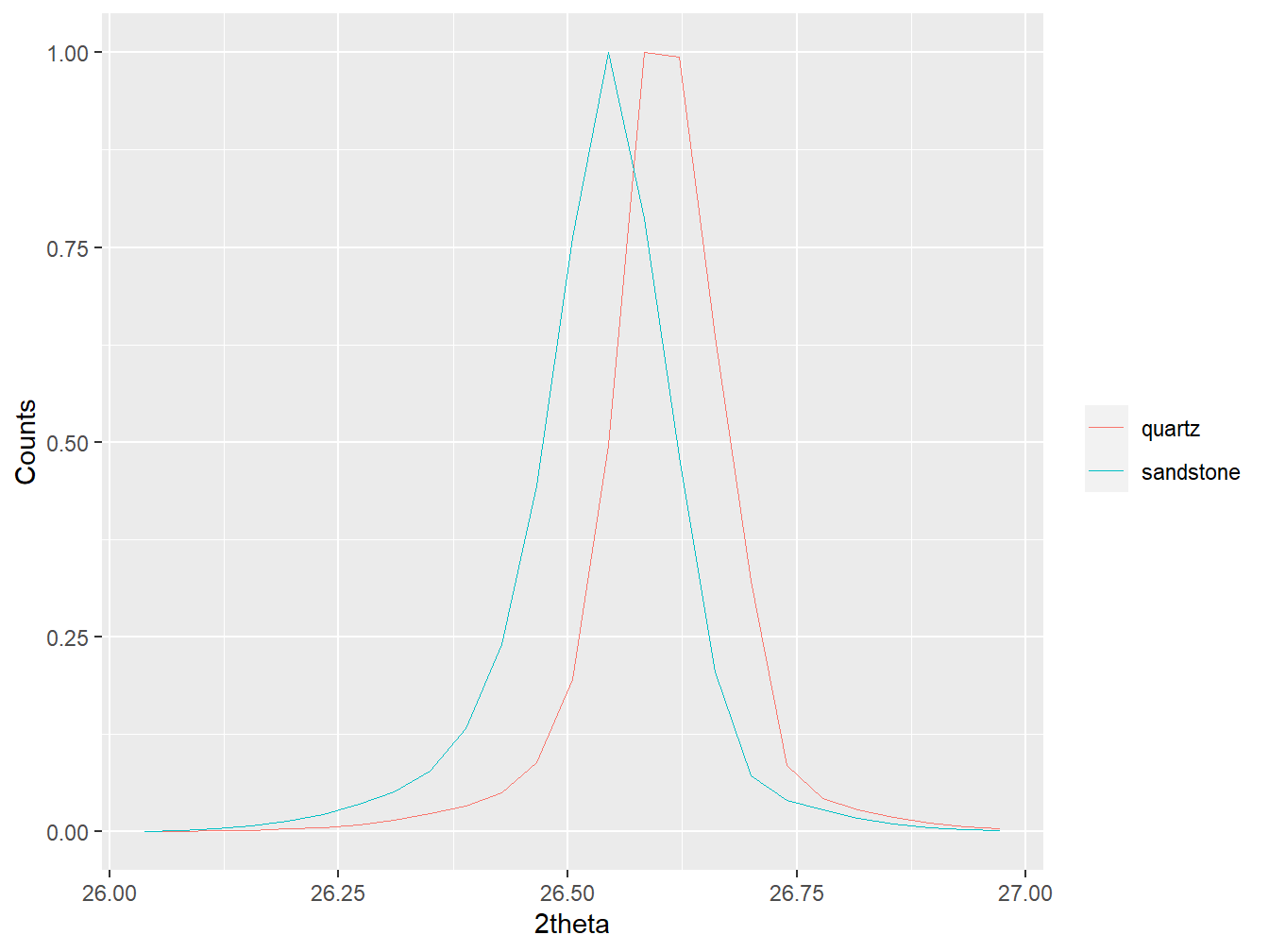
Figure 1.11: Unaligned diffractograms.
As shown in the figure above, the main quartz peaks of these two diffraction patterns do not align. This can be corrected using align_xy():
#Align the sandstone soil to the quartz pattern
sandstone_aligned <- align_xy(soils$sandstone, std = quartz,
                              xmin = 10, xmax = 60, xshift = 0.2)

#Plot the main quartz peak for pure quartz and a sandstone-derived soil
plot(as_multi_xy(list("quartz" = quartz,
                      "sandstone aligned" = sandstone_aligned)),
     wavelength = "Cu",
     normalise = TRUE,
     xlim = c(26, 27))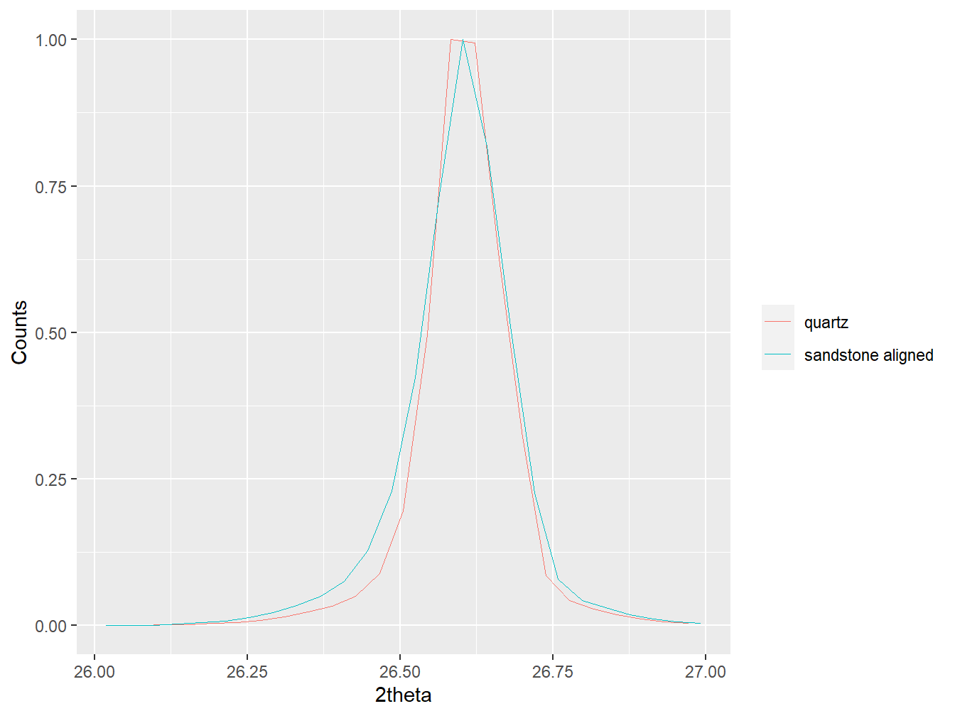
Figure 1.12: Aligned diffractograms.
In cases where multiple patterns require alignment to a given standard, align_xy() can also be applied to multiXY objects:
#Plot the unaligned soils data to show misalignments
plot(soils, wav = "Cu",
     xlim = c(26, 27), normalise = TRUE)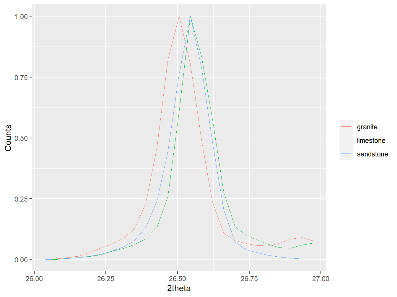
Figure 1.13: Unaligned diffractograms in a multiXY object.
#Align the soils data to the quartz pattern
soils_aligned <- align_xy(soils, std = quartz,
                          xmin = 10, xmax = 60, xshift = 0.2)

#Plot the aligned data
plot(soils_aligned,
     wavelength = "Cu",
     normalise = TRUE,
     xlim = c(26, 27))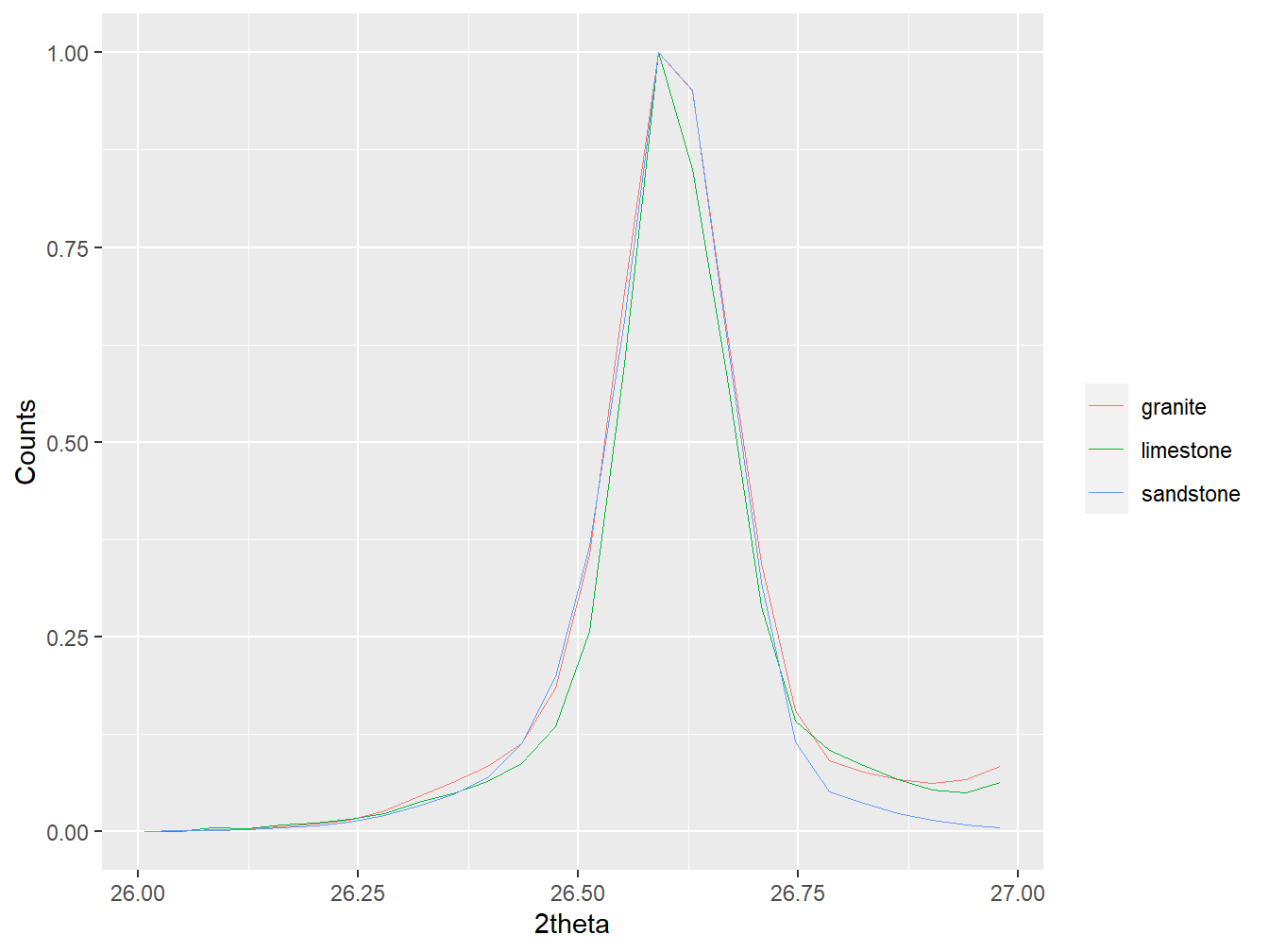
Figure 1.14: Aligned diffractograms in a multiXY object.
1.4.5 Background fitting
Sometimes it is beneficial to fit and subtract the background from XRPD data. To achieve this, the powdR package includes the bkg() function which uses the peak filling method implemented in the baseline package (Liland, Almøy, and Mevik 2010). The fitting provided by the bkg() function uses four adjustable parameters that each have pre-loaded defaults (see ?bkg):
#Fit a background to the sandstone-derived soil
granite_bkg <- bkg(soils$granite)

#summarise the resulting data
summary(granite_bkg)
## Length Class Mode
## tth 1693 -none- numeric
## counts 1693 -none- numeric
## background 1693 -none- numeric#Plot the data and add a square root transform to aid interpretation
plot(granite_bkg) +
scale_y_sqrt()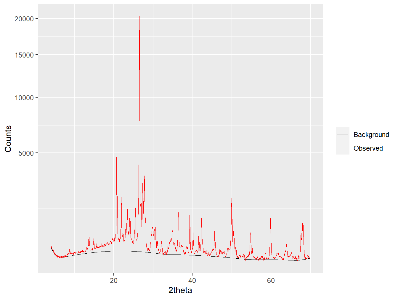
Figure 1.15: Fitting a background to a soil diffractogram. The y-axis is square root transformed to aid interpretation.
It is then simple to derive a background-subtracted XY object:
#Calculate background subtracted count intensities
sandstone_bkg_sub <- as_xy(data.frame("tth" = granite_bkg$tth,
                                      "counts" = granite_bkg$counts -
                                                 granite_bkg$background))

plot(sandstone_bkg_sub, wavelength = "Cu")
Figure 1.16: Background subtracted diffractogram.
Sometimes the default values for the adjustable parameters (see ?bkg) are not appropriate, and in such cases tuning of the parameters can be an iterative process. To help with this, there is a background fitting Shiny app that can be loaded from the powdR package using run_bkg(). This app will load in your default web browser and allows for the four adjustable parameters to be tuned to a given sample that is loaded into the app in ‘.xy’ format.
1.4.6 Converting to and from data frames
multiXY objects can be converted to data frames using the multi_xy_to_df() function. When using this function, all samples within the multiXY object must be on the same 2θ axis, which can be ensured using the interpolate() function outlined above.
#Convert xy_list1 to a dataframe
xy_df1 <- multi_xy_to_df(xy_list1, tth = TRUE)

#Show the first 6 rows of the derived data frame
head(xy_df1)
## tth D5000_1 D5000_2 D5000_3 D5000_4 D5000_5
## 1 2.00 2230 2334 2381 2323 2169
## 2 2.02 2012 2222 2297 2128 2021
## 3 2.04 1950 2031 2211 2056 1929
## 4 2.06 1828 1972 2077 1918 1823
## 5 2.08 1715 1896 2000 1861 1757
## 6 2.10 1603 1701 1868 1799 1673In cases where the 2θ column is not required, the use of tth = FALSE in the function call will result in only the count intensities being included in the output.
Data frames that take the form of xy_df1 (i.e. that include the 2θ axis) can easily be converted back to a multiXY object using as_multi_xy():
#Convert xy_df1 back to a multiXY list
back_to_list <- as_multi_xy(xy_df1)

#Check the class of the converted data
class(back_to_list)
## [1] "multiXY" "list"1.4.7 2θ transformation
Laboratory XRPD data are usually collected using either Cu or Co X-ray tubes, and the main component of the emission profile from these is the characteristic Kα wavelengths (e.g. Cu-Kα = 1.54056 Angstroms whereas Co-Kα = 1.78897 Angstroms). These wavelengths determine the 2θ at which the conditions for diffraction are met via Bragg’s Law:
\[ \begin{aligned} n\lambda = 2d\sin\theta \end{aligned} \]
where \(n\) is an integer describing the diffraction order, \(\lambda\) is the wavelength (Angstroms) and \(d\) is the atomic spacing (Angstroms) between repeating planes of atoms in a crystal (mineral).
In some instances it can be useful to transform the 2θ axis of a given sample so that the 2θ peak positions are representative of a measurement made using a different X-ray source. This can be achieved using the tth_transform() function:
#Create a multiXY object for this transform example
transform_eg <- as_multi_xy(list("Co" = xy_list1$D5000_1,
                                 "Cu" = soils$sandstone))

#Plot two patterns recorded using different wavelengths
plot(transform_eg,
     wavelength = "Cu",
     normalise = TRUE,
     interactive = FALSE)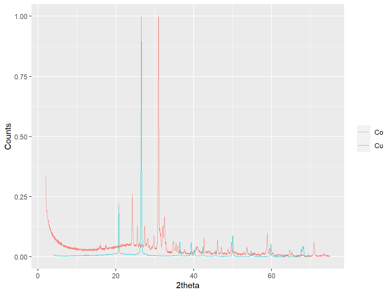
Figure 1.17: Data obtained from Co and Cu X-ray tubes prior to 2theta transformation.
#transform the 2theta of the "Co" sample to "Cu"
transform_eg$Co$tth <- tth_transform(transform_eg$Co$tth,
                                     from = 1.78897,
                                     to = 1.54056)

#Replot data after transformation
plot(transform_eg,
     wavelength = "Cu",
     normalise = TRUE,
     interactive = FALSE)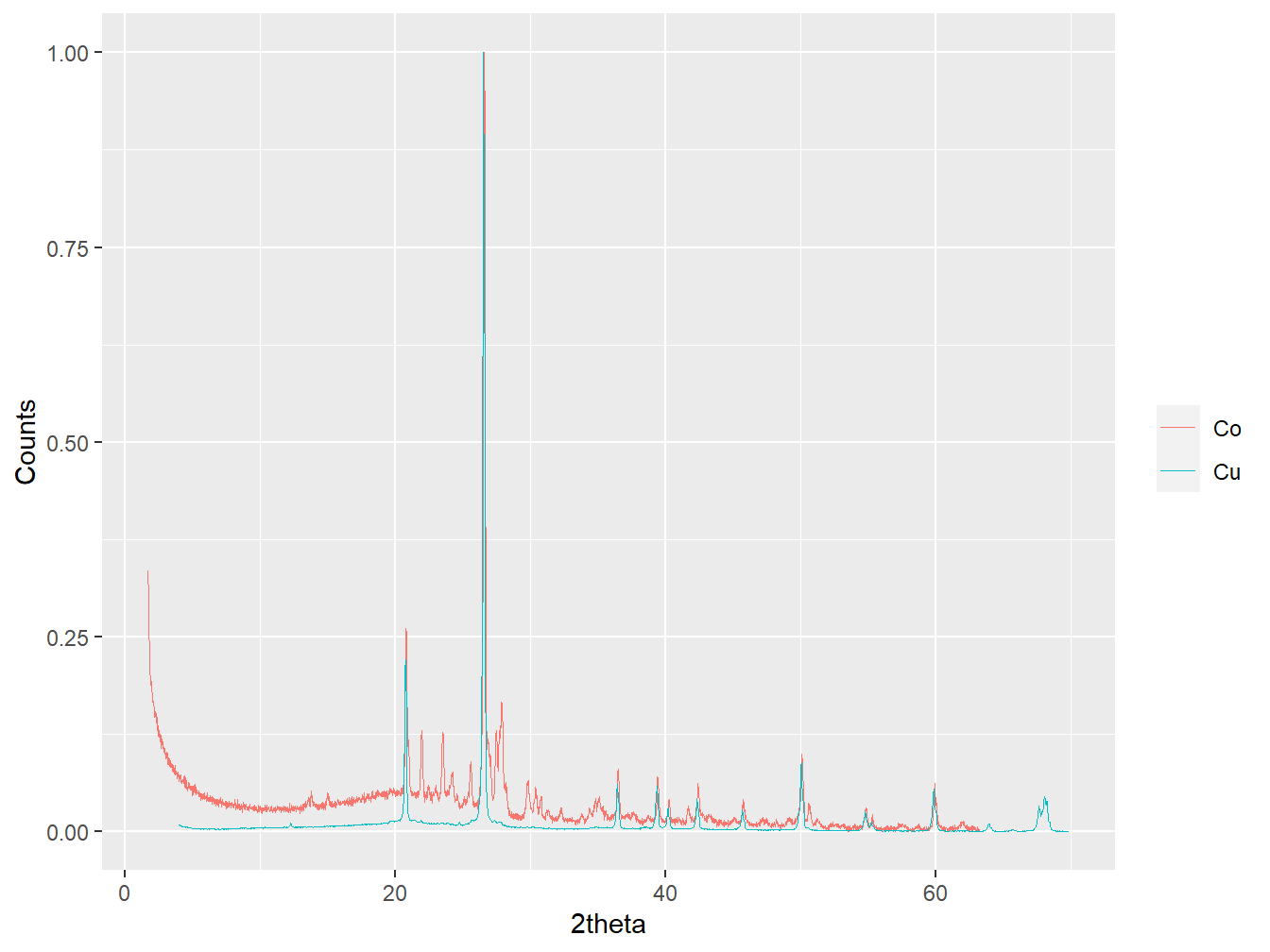
Figure 1.18: Data obtained from Co and Cu X-ray tubes after 2theta transformation.
Note how prior to the 2θ transformation, the dominant peaks in each pattern (associated with quartz in both cases) do not align. After the 2θ transformation the peaks are almost aligned, with a small additional 2θ shift that could be computed using the align_xy() function outlined above. Whilst Cu and Co are the most common X-ray sources for laboratory diffractometers, tth_transform() can accept any numeric wavelength value.