Chapter 3 Machine learning with soil XRPD data
This chapter will demonstrate the use of the Cubist machine learning algorithm to predict and interpret soil properties from XRPD data. Cubist is an extension of Quinlan’s M5 model tree (Quinlan 1992), and is featured in the CRAN repository under the same name for use in the R statistical software environment (Kuhn and Quinlan 2022). Cubist defines a series of conditions based on predictor variables (i.e. the XRPD measurement intervals) that partition the data. At each partition there is a multivariate linear model used to predict the output (i.e. the soil property).
The examples presented herein for the use of Cubist will use data from Butler et al. (2020) that is hosted on Mendeley Data here. More specifically, to run the examples in this chapter on your own machine, you will need to download the soil property data in ‘.csv’ format and the XRPD data in a zipped folder of ‘xy’ files. Please simply save these files to your own directory, and unzip the zipped folder containing the ‘.xy’ files.
3.1 Loading packages and data
This chapter will use a number of packages that should already be installed on your machine, but will also use the leaflet and Cubist packages that may need to be installed if you have not used them before:
#install packages that haven't been used on this course so far
install.packages(c("leaflet" and "Cubist"))
#load the relevant packages
library(powdR)
library(leaflet)
library(ggplot2)
library(Cubist)
library(plotly)Once you have loaded the packages and downloaded the data required for this chapter, the data can be loaded into R by modifying the paths in the following code:
#Load the soil property data
props <- read.csv(file = "path/to/your/file/clusters_and_properties.csv")

#Get the full file paths of the XRPD data
xrpd_paths <-  dir("path/to/xrd", full.names = TRUE)

#Load the XRPD data
xrpd <- read_xy(files = xrpd_paths)

#Make sure the data are interpolated onto the same 2theta scale
#as there are small differences within the dataset
xrpd <- interpolate(xrpd, new_tth = xrpd$icr030336$tth)
3.2 Data exploration
The dataset used in this chapter is comprised of 935 sub-soil samples from sub-Saharan Africa, sampled as part of the AfSIS Sentinel Site programme using the Land Degradation Surveillance Framework. A range of soil attributes and properties are provided in the props data, whilst each item within the xrpd data is an XY diffractogram of the soil. The names of xrpd data match the unique identifiers in the props$SSN column:
#Check that the names of the xrpd data match the SSN column in props
identical(names(xrpd), props$SSN)
## [1] TRUE3.2.1 Spatial data
The first 4 columns of the props data include the unique SSN identifier of each sample, the name of the Sentinel Site, and the sample location (Longitude and Latitude). Initial exploration of the spatial distribution of the dataset can be achieved using the leaflet package (Cheng, Karambelkar, and Xie 2022). A detailed guide of how to use leaflet in R is beyond the scope of this documentation, but the code used below can be adapted to produce basic plots of geo-referenced point data. leaflet maps are built up in layers similar to the principle of ggplot2 figures, with each layer being separated by a %>%, which can be written in R using the Ctrl+Shift+M shortcut.
leaflet(props) %>% #create a leaflet object from props
  addTiles() %>% #add the default tiles for the map surface
  addCircleMarkers(~Longitude, ~Latitude)
Figure 3.1: Interactive map of the Sentinel Site data showing all 60 sites across sub-Saharan Africa.
The map resulting from the above code shows the 60 Sentinel Sites within the dataset that together account for many of the agro-ecological regions of sub-Saharan Africa. By zooming in on the Sentinel Sites individually, it can be observed that each is comprised of a random grid of up to 16 samples within a 10 x 10 km area (Butler et al. 2020):
leaflet(props[props$Sentinel_site == "Bana",]) %>%
  addTiles() %>%
  addCircleMarkers(~Longitude, ~Latitude)
Figure 3.2: Interactive map of the Bana Sentinel Site showing the sixteen sampling locations within the 10 x 10 km grid.
3.2.2 Geochemical data
The props data contains a wide range of geochemical variables including pH, total organic carbon (TOC), total element concentrations (columns 9 to 15) and Mehlich-3 extractable element concentrations (columns 16 to 23). The examples provided in this chapter will focus on total concentrations of K, determined using X-ray Fluorescence (Butler et al. 2020), but the code can be easily adjusted for any other soil property within the dataset.
Here the K concentration data will be summarised using the summary() function plotted as a histogram using ggplot2:
#summarise the K concentration data
summary(props$K)
## Min. 1st Qu. Median Mean 3rd Qu. Max.
## 90.41 2482.09 7045.57 11535.65 16947.73 95674.79#Produce a histrogram of the log transformed K data
ggplot(data = props, aes(log(K))) +
geom_histogram()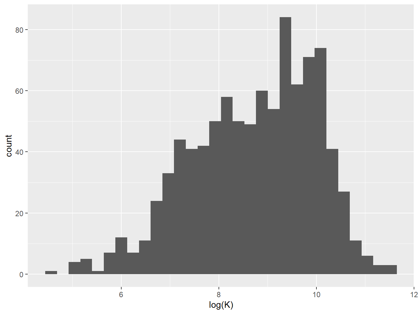
Figure 3.3: Histogram of total K concentrations (log transformed)
3.2.3 XRPD data
Given there are 935 diffractograms within the xrpd data, it is not possible to visually inspect all data at once. To start with, it is probably worth visualising the diffractograms from one Sentinel site at a time.
plot(as_multi_xy(xrpd[props$SSN[props$Sentinel_site == "Didy"]]),
     wavelength = "Cu",
     normalise = TRUE)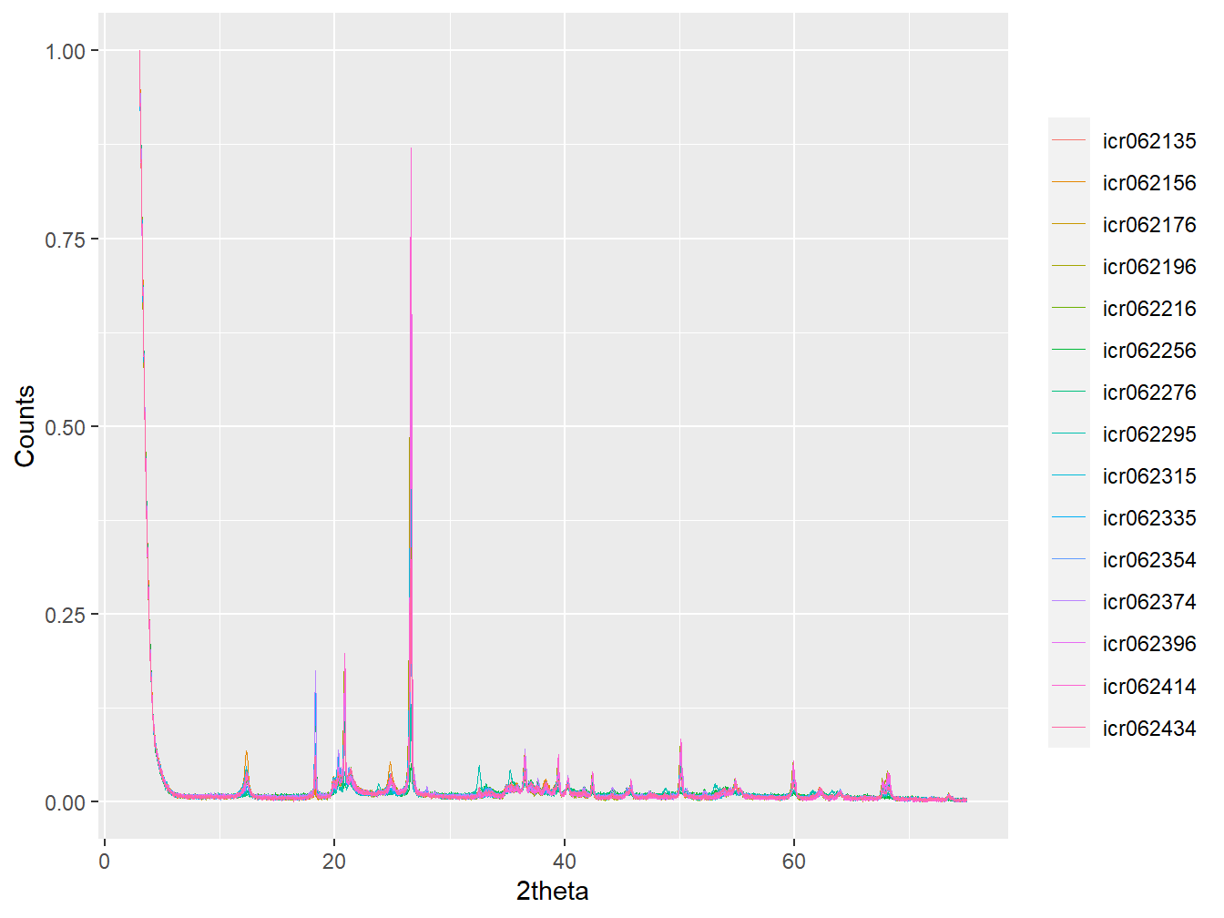
Figure 3.4: Diffractograms associated with the Didy site.
Visualising the data in this way shows how the strongest peak in each diffractogram at the ‘Didy’ Sentinel Site occurs at approximately 26 \(^\circ\) 2θ. Further inspection of this peak shows how there are minor adjustments in alignment that will need to be applied to the data:
plot(as_multi_xy(xrpd[props$Sentinel_site == "Didy"]),
     wavelength = "Cu",
     normalise = TRUE,
     xlim = c(26,27))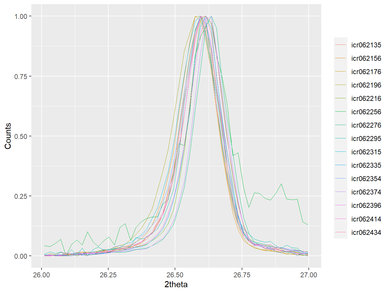
Figure 3.5: The major quartz peak of the diffractograms associated with the Didy site, highlighting small 2theta misalignments.
This strong peak is associated with quartz, which is omnipresent in soil datasets like this and is a strong diffractor of X-rays. Together this results in quartz peaks being the dominant signal in most soil diffractograms, which is a feature that can be particularly useful for peak alignment when pre-treating the data.
3.3 Data pre-treatment
Prior to applying Cubist to the XRPD data, it is important to apply corrections for sample-independent variation such as small 2θ misalignments and/or fluctuations in count intensities.
3.3.1 Alignment
The small 2θ misalignments identified above can be corrected for using the align_xy() function in powdR. Quartz is omnipresent within the dataset and therefore the samples can be aligned to a pure quartz pattern. A pure quartz pattern can be created from the rockjock library, and then used for sample alignment within a restricted 2θ range.
#Extract a quartz pattern from rockjock
quartz <- as_xy(data.frame(rockjock$tth,
                           rockjock$xrd$QUARTZ))

plot(quartz, wavelength = "Cu")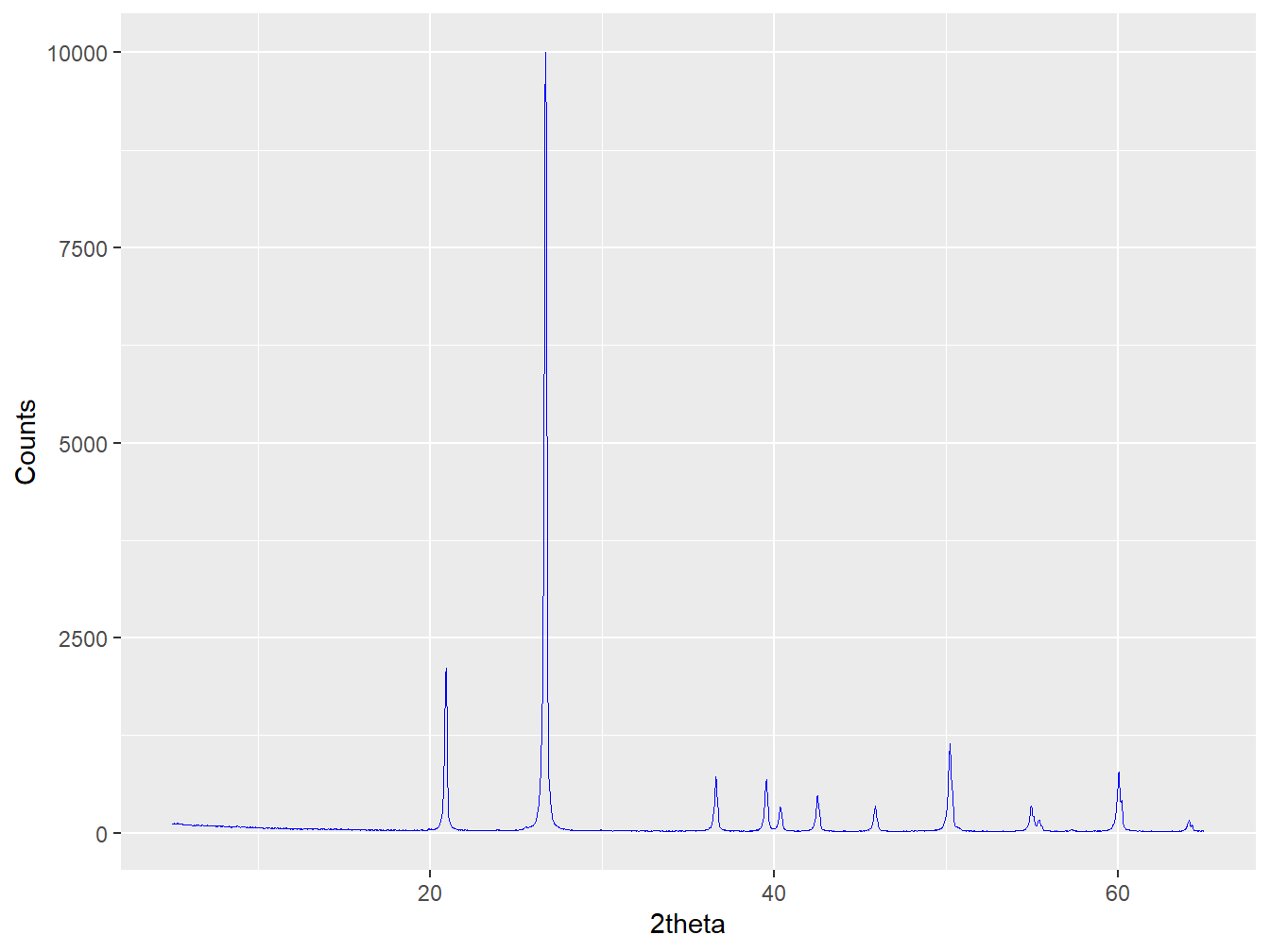
Figure 3.6: A pure quartz pattern extracted from the rockjock reference library.
#Align the xrpd data to this quartz pattern
#using a restricted 2theta range of 10 to 60
xrpd_pt <- align_xy(xrpd, std = quartz,
                    xmin = 10, xmax = 60,
                    xshift = 0.2)

plot(as_multi_xy(xrpd_pt[props$Sentinel_site == "Didy"]),
     wavelength = "Cu",
     normalise = TRUE,
     xlim = c(26,27))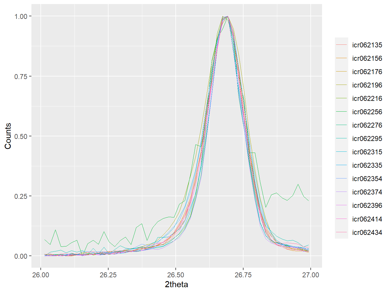
Figure 3.7: Diffractograms from the Didy site aligned to the quartz pattern extracted from the rockjock reference library.
Alignment of the data in this way is important because even seemingly small misalignments between peaks can hinder the comparison of XRPD data by multivariate methods, and hence reduce the effectiveness of the analysis (Butler et al. 2019).
3.3.2 Subsetting
In Figure 3.4 it can be observed that below ~4 \(^\circ\) 2θ there is a tall tail in count intensities. This tail, probably due to the detector starting to ‘see’ the direct beam form the X-ray source, can be removed by subsetting the data using the code described above.
xrpd_pt <- lapply(xrpd_pt, subset,
                  tth >= 5 & tth <= 75)

plot(as_multi_xy(xrpd_pt[props$Sentinel_site == "Didy"]),
     wavelength = "Cu")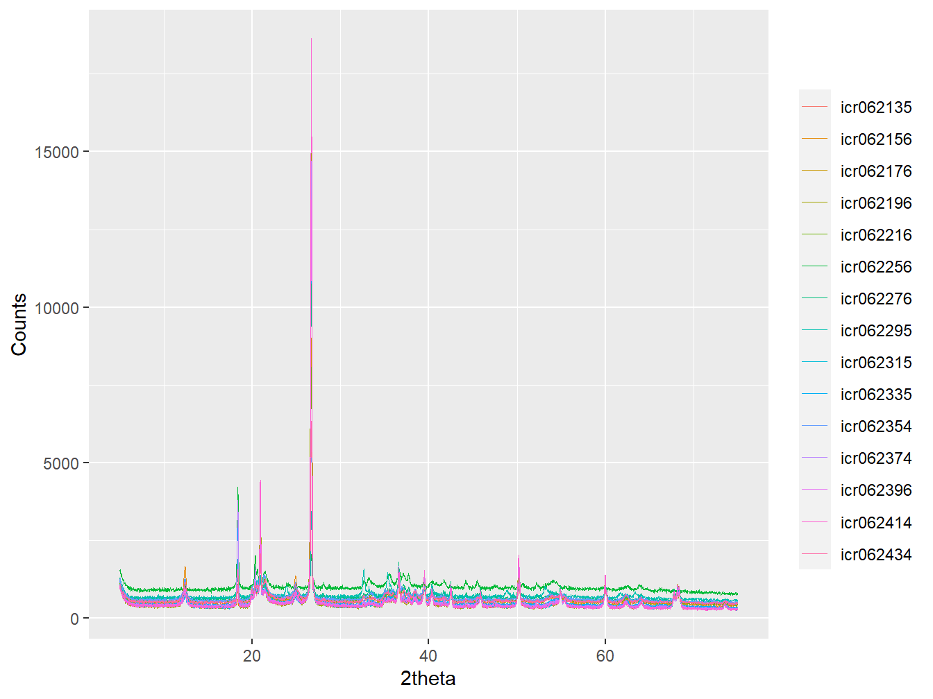
Figure 3.8: Aligned diffractograms subset to remove data below 5 degrees 2theta.
3.3.3 Mean centering
In addition to alignment and subsetting, it can be useful to adjust the data for fluctuating count intensities that can be associated with factors such as the natural deterioration of the X-ray source over time. Such adjustment can be achieved by mean centering, which subtracts the mean from the count intensities of each sample:
#Create a mean centering function
mean_center <- function(x) {

  x[[2]] <- x[[2]] - mean(x[[2]])

  return(x)

}

#apply the function to all patterns
xrpd_pt <- lapply(xrpd_pt, mean_center)

#Inspect the data from Didy
plot(as_multi_xy(xrpd_pt[props$Sentinel_site == "Didy"]),
     wavelength = "Cu")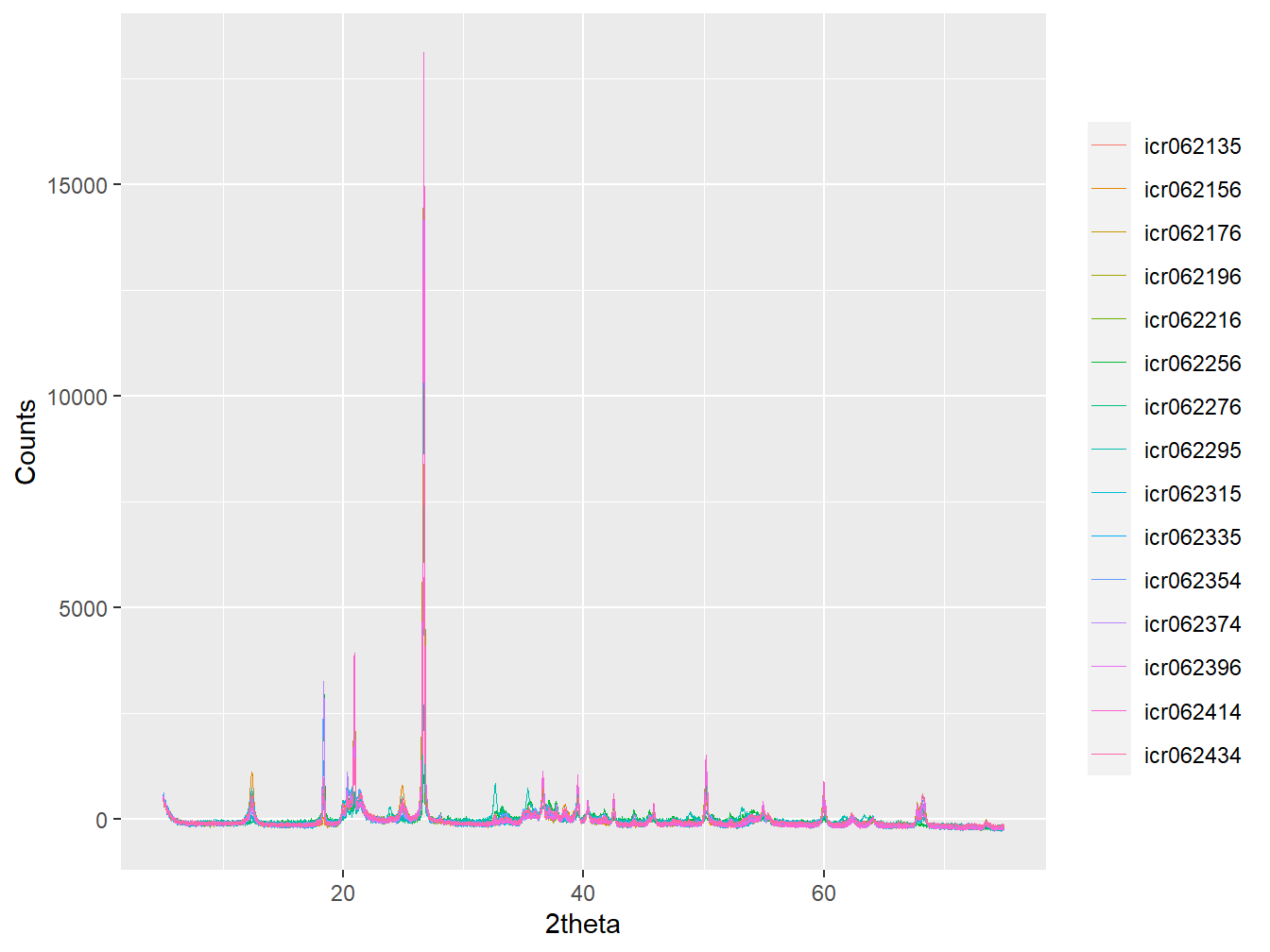
Figure 3.9: Aligned, subset and mean centred diffractograms.
Now we are left with the dataset xrpd which consists of 935 diffractograms that have each been aligned, subset and mean centred. At this point we are ready to apply the Cubist algorithm to the data.
3.4 Creation of training and test datasets
Cubist is a supervised machine learning algorithm and therefore requires training using a dataset that accounts for much of the variation that may be observed in the dataset that Cubist predicts a given soil property from.
Here, 75 % of the data will be used as a training set for Cubist to develop appropriate decisions and regression models from, hereafter, the training dataset. The remaining 25 % of the data will be used to test the accuracy of the derived models on ‘new’ data (i.e. data that was not used to train the model), hereafter, the test dataset.
There are a range of different approaches for defining the training and test datasets. Here a purely random approach will be employed using the sample() function:
#Set the seed for random number generation
#so that results are reproducible.
set.seed(10)

#Randomly select 75% of the samples
selection <- sample(1:nrow(props),
                    size = round(nrow(props)*0.75),
                    replace = FALSE)
3.5 Using Cubist
Here Cubist will be applied to the XRPD data in order to predict and interpret total K concentrations. Underpinning this approach is the principle that a soil diffractogram represents a reproducible signature of that soil’s mineral composition, and the mineral composition is a key controller of total K concentrations. The code can be readily adapted to any of the other properties within the data, or to your own soil XRPD data and associated properties.
To run Cubist the XRPD data need to be supplied in dataframe format, with each row of the dataframe representing a sample. The XRPD data can easily be converted to a dataframe using the multi_xy_to_df function outlined above:
#double check that the order of xrpd and props
#data match
identical(names(xrpd_pt), props$SSN)
## [1] TRUE#create a data frame
xrpd_df <- multi_xy_to_df(as_multi_xy(xrpd_pt),
tth = TRUE)
#transpose the data so that each sample is a row
cubist_xrpd <- data.frame(t(xrpd_df[-1]))There are a couple of parameters that can be adjusted when training Cubist models: committees and neighbours (see Butler, O’Rourke, and Hillier (2018)). Various routines exist for tuning these parameters in order to produce the most accurate models. For further reading on this tuning process, see the documentation for the caret and Cubist packages.
For simplicity, the adjustable Cubist parameters used in this example will be set to committees = 10 when training the models, and neighbours = 9 when using the derived models to predict total K concentrations from new data. The Cubist models can be trained using the training dataset using:
#Create a Cubist model for K
cubist_K <- cubist(x = cubist_xrpd[selection,],
                   y = props$K[selection],
                   committees = 10)
following which, the derived models can be used to predict the total K concentrations from XRPD data in the test dataset:
#Predict K
predict_K <- predict(cubist_K,
                     cubist_xrpd[-selection,],
                     neighbours = 9)

#Plot measured K vs predicted K
plot(x = log(props$K[-selection]), log(predict_K),
     xlab = "log(Measured K), ppm", ylab = "log(Predicted K), ppm")
abline(0,1) #Add a 1:1 line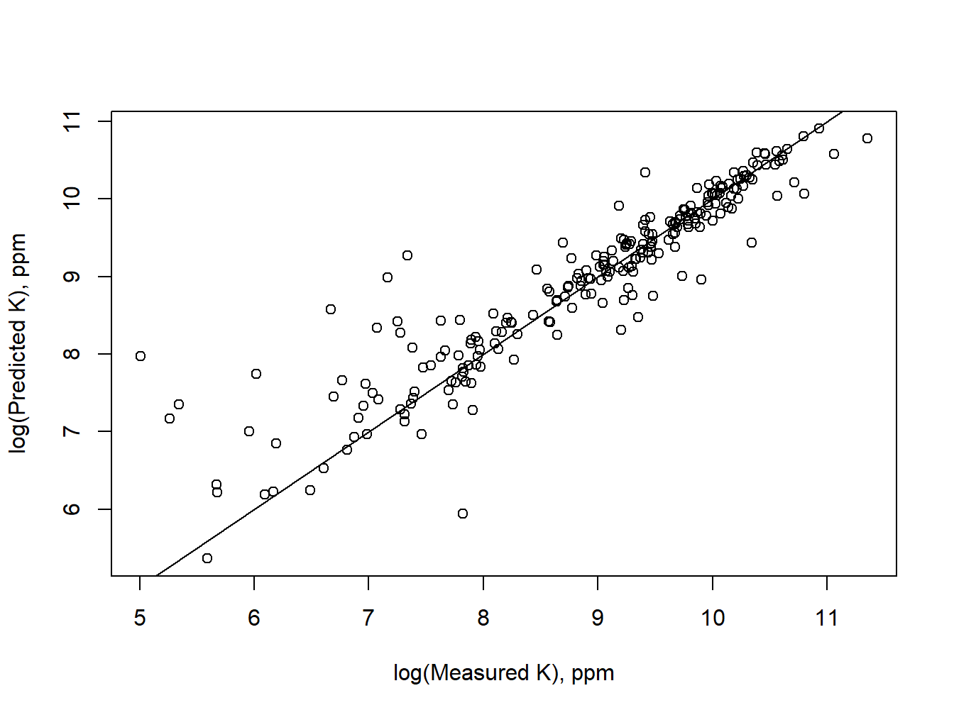
#R2 of measured K vs predicted K
cor(log(props$K[-selection]), log(predict_K))^2
## [1] 0.8540419The Cubist model for K prediction therefore results in a relatively accurate prediction of K, with an \(R^2\) of ~0.85. This indicates that Cubist is able to extract appropriate variables from the XRPD data and use them to predict chemical soil properties.
3.6 Inspection of Cubist models
The variables that Cubist selects can be plotted in order to decipher the mineral contributions to a given soil property:
#Extract the usage data from the Cubist model
K_usage <- cubist_K$usage

#Make sure the variable names are numeric so that they can be ordered
K_usage$Variable <- as.numeric(substr(K_usage$Variable,
                                      2,
                                      nchar(K_usage$Variable)))

#Order the K_usage data by Variable now it is numeric
K_usage <- K_usage[order(K_usage$Variable), ]

#Add the 2theta axis
K_usage$tth <- xrpd_df$tth

#Add a mean diffracotgram to the data
K_usage$counts <- rowMeans(xrpd_df[-1])

#Create a function that normalises a vector data to a minimum of 0
#and maximum of 1.
range01 <- function(x){(x-min(x))/(max(x)-min(x))}

#Create the plot
ggplot(data = K_usage) +
geom_linerange(aes(x = tth, ymax = Model/100, ymin = 0),
               colour = "grey81", size = 1) +
geom_linerange(aes(x = tth, ymax = Conditions/100, ymin = 0),
               colour = "grey19", size = 1) +
geom_line(aes(x = tth, y = range01(counts)), colour = "red",
          size = 0.5) +
ylab("Scaled counts and fraction of variable use\n") +
xlab("2theta") +
theme_bw()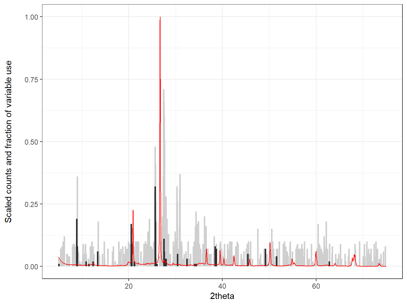
Figure 3.10: Features selected by Cubist for the prediction of K. Grey sticks denote the fraction of variable use in the regression models and black sticks denote the fraction of variable use in decision. Red line is the mean diffractogram for the dataset.
Figure 3.10 shows how the most important variables for prediction of K concentrations are found between 25 and 30 \(^\circ\) 2θ. To further aid with interpretation of such regions, these plots can be combined with data from full pattern summation so that the variables selected by Cubist can be attributed to specific minerals. For example:
f1 <- fps(lib = rockjock,
          smpl = xrpd$icr014764,
          std = "QUARTZ",
          refs = c("K-feldspar",
                   "Quartz",
                   "Mica (Tri)",
                   "Organic matter",
                   "Halloysite",
                   "Kaolinite",
                   "Rutile",
                   "Background"),
          align = 0.2)
##
## -Harmonising library to the same 2theta resolution as the sample
## -Aligning sample to the internal standard
## -Interpolating library to same 2theta scale as aligned sample
## -Optimising...
## -Removing negative coefficients and reoptimising...
## -Removing negative coefficients and reoptimising...
## -Removing negative coefficients and reoptimising...
## -Computing phase concentrations
## -Internal standard concentration unknown. Assuming phases sum to 100 %
## ***Full pattern summation complete***yields a reasonable fit of the data, as can be inspected using plot(f1, wavelength = "Cu", interactive = TRUE). To help identify what minerals the variables between 25 and 30 \(^\circ2\) 2θ are associated with, the results in f1 can be combined with the results in K_usage:
#Create a plot of the full pattern summation results
p1 <- plot(f1, wavelength = "Cu", group = TRUE)

#Define the layers for the sticks that will have to be placed
#BENEATH the data in p1
p2 <- geom_linerange(data = K_usage,
                     aes(x = tth,
                         ymax = (Model/100)*max(f1$measured),
                         ymin = 0),
                     colour = "grey81", size = 1)

p3 <- geom_linerange(data = K_usage,
                     aes(x = tth,
                         ymax = (Conditions/100)*max(f1$measured),
                         ymin = 0),
                     colour = "grey19", size = 1)

#Order the layers so that p2 and p3 are beneath p1
p1$layers <- c(p2, p3, p1$layers)

#Limit the x-axis to between 25 and 30 degrees so that the
#dominant features can be easily examned
p1 <- p1 +
      scale_x_continuous(limits = c(25, 30))

p1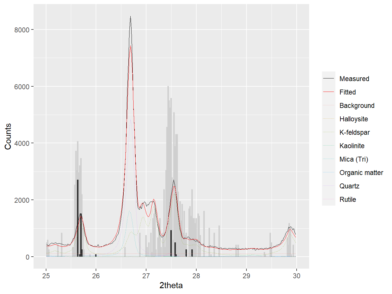
Figure 3.11: Combining the results from full pattern summation with the features selected by Cubist for prediction of K concentrations.
To make the data in Figure 3.11 interactive, it’s possible to use the ggplotly() function of the plotly package via:
ggplotly(p1)From these plots (in particular the interactive version), it is possible to infer that the variables selected by Cubist in this region are specifically related to K-feldspar contributions to the diffraction data. K-feldspar minerals represent the major K-reserves in most soils (though the availability of its potassium to plants is a different matter) and this selection by Cubist is therefore completely appropriate. Further potential mineral sources of other nutrients and micronutrients within this or other datasets can be inferred in a similar manner.