Chapter 5 From Mars to Mull: Interplanetary comparison of soil XRPD data
This chapter will use data from the Mars Science Laboratory (MSL) onboard NASA’s Curiosity Rover. The MSL XRPD data were obtained from the Geosciences Data Volume Online as ASCII ‘.csv’ files on the 17th July 2021 and loaded into R (Vaniman 2012) using read.csv().
The mineral compositions of the samples in the MSL dataset are described and discussed in numerous publications (Bish et al. 2013; Grotzinger et al. 2014; Vaniman et al. 2014; Bristow et al. 2015, 2018). The many clay minerals identified and quantified from the XRPD data provides compelling evidence that the Martian surface material has been altered by water, which has profound implications for the potential existence of microbial life on Mars.
Qualitative and quantitative analysis of clay minerals is a notoriously challenging undertaking, often requiring separation of the clay fraction onto oriented slides combined with treatements such as ethylene-glycol solvation and heating, among others. The MSL cannot separate the clay fraction from Martian samples and is limited to bulk sample analysis, where clay minerals are analysed in a randomly oriented powder along with all other crystalline and amorphous components within the sample. This has acted to create some uncertainty in the analysis of clay minerals from MSL XRPD data (Bish et al. 2013; Grotzinger et al. 2014; Vaniman et al. 2014; Bristow et al. 2018). Identification of Earth based analogues for Martian soil mineralogy therefore represent an opportunity to facilitate more accurate interpretation of the clay mineralogy encoded within MSL XRPD data. Further, understanding the development of mineralogically analogous soils on Earth has potential to aid the development of hypotheses for the environmental properties of aqueous systems on ancient Mars (Marlow, Martins, and Sephton 2008).
Here, soil XRPD data from across Scotland (Butler, O’Rourke, and Hillier 2018) will be compared to the MSL XRPD data with the aim of identifying potential soil analogues for Martian mineralogy.
5.1 Required packages
Data for this chapter are stored within a mars2mull R package hosted on GitHub. The package can be installed using the devtools package
#Install devtools if it's not already on your machine
install.packages("devtools")

#Use devtools to install the mars2mull package from GitHub
devtools::install_github("benmbutler/mars2mull")
Running the code for this chapter requires the mars2mull package along with a few other packages that have already been introduced and used in previous Chapters of this course:
library(mars2mull)
library(powdR)
library(ggplot2)
library(leaflet)
5.2 Datasets
5.2.1 Mars Science Laboratory XRPD Data
Martian XRPD data within the package have been extracted from NASA’s Geosciences Data Volume Online (Vaniman 2012) and renamed according to the various sites that were sampled. The diffractograms of 31 Martian samples are contained within the mars_xrpd data in multiXY format. All diffractograms were collected using Co-Kα radiation, with further details of the data collection and instrumental parameters provided elsewhere (Bish et al. 2013; Grotzinger et al. 2014; Vaniman et al. 2014; Bristow et al. 2015, 2018). Upon loading the mars_xrpd data here, we will subset the diffractograms to 2θ >= 4.5 degrees in order to remove the contributions from the sample holder at low angles:
#load the Martian XRPD data
data(mars_xrpd)

#Subset the Martian XRPD data to >4.5
#to avoid single from sample holder
mars_xrpd <- as_multi_xy(lapply(mars_xrpd, subset,
                                tth >= 4.5))

#plot the 31 Martian diffractograms
plot(mars_xrpd, wavelength = "Co",
     normalise = TRUE, interactive = FALSE)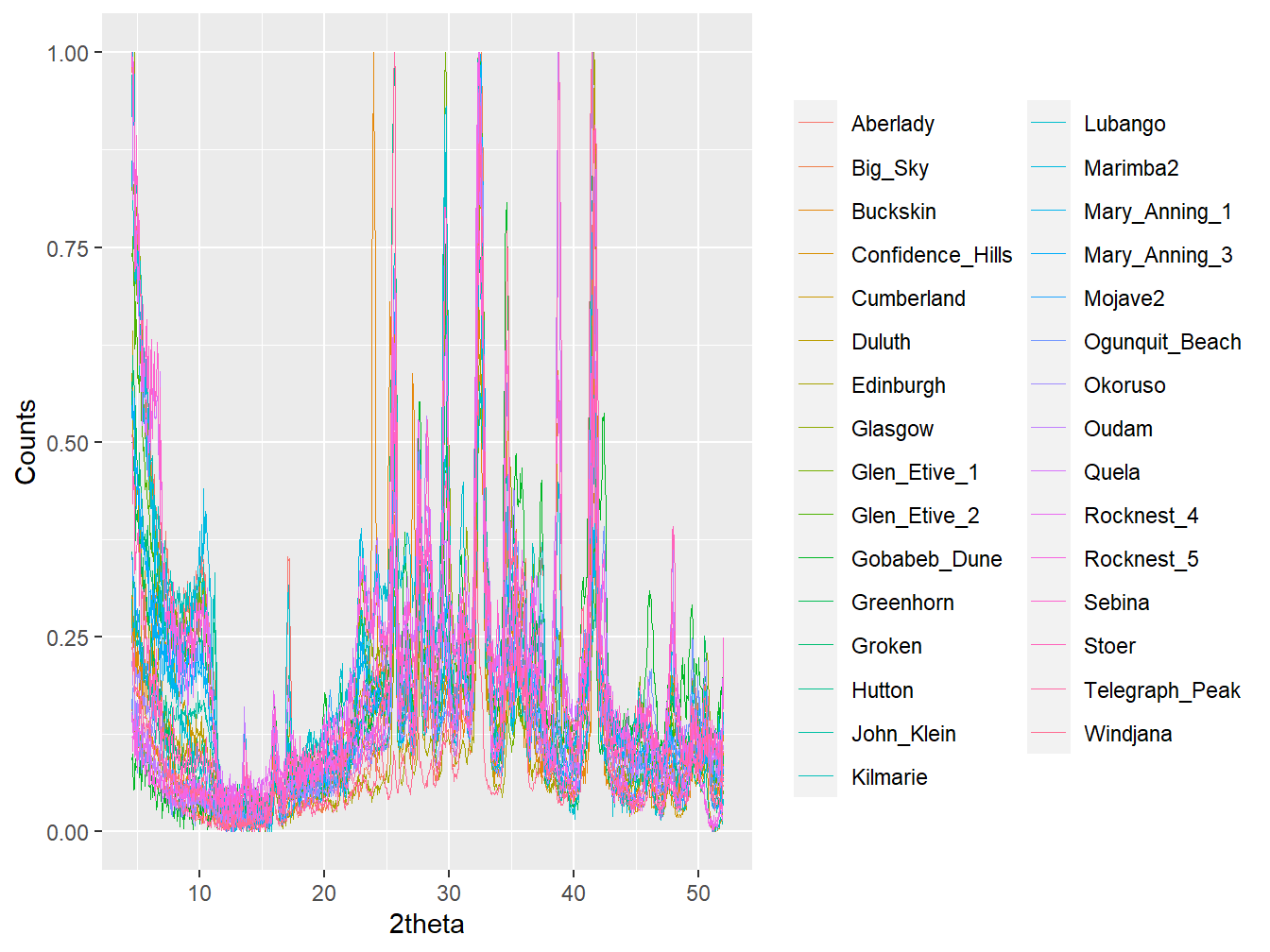
Figure 5.1: The 31 diffractograms within the mars_xrpd data. Using interactive = TRUE in the function call will allow for easier interpretation.
Further to the XRPD data, additional information about each of the samples is provided in the mars_id data, and more help can be accessed via ?mars_id:
#load the extra information about the samples interactively
data(mars_id)

#View the first 6 rows of the mars_id data
head(mars_id)
## SITE_NAME PRODUCT_ID SAMPLE_TYPE SOL_START
## 1 Rocknest_4 cma_404470826rda00790050104ch11503p1 Scoop 77
## 2 Rocknest_5 cma_405889312rda00950050104ch11504p1 Scoop 94
## 3 Cumberland cmb_434685266rda04190180786ch00113p1 Drill 418
## 4 John_Klein cmb_439549561rda04740240192ch00111p1 Drill 473
## 5 Windjana cmb_452848863rda06240311330ch00111p1 Drill 623
## 6 Confidence_Hills cmb_465487684rda07660421020ch00113p2 Drill 765
## SOL_END
## 1 88
## 2 119
## 3 432
## 4 488
## 5 632
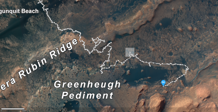
## 6 785The locations of the 31 samples can be explored using the SOL_START and SOL_END columns in the mars_id data in combination with NASA’s online map for Curiosity’s location (screenshot below).
5.2.2 Scottish Soil XRPD data
The Scottish soil diffractograms relate to 703 samples collected by horizon from 186 sites across Scotland. Samples were collected primarily as part of the second National Soil Inventory of Scotland (NSIS, Butler, O’Rourke, and Hillier 2018) and are supplemented by additional samples of rare Scottish soils. Information about the samples is provided in the scotland_locations data:
#Load the scotland_locations data
data(scotland_locations)

#Show the first 6 rows of the data
head(scotland_locations)
## SAMPLE_ID PROFILE_ID PROFILE_LONGITUDE PROFILE_LATITUDE
## 72 S891338 S13735 -3.004763 57.62634
## 73 S891345 S13516 -3.004763 57.62620
## 74 S891346 S13516 -3.004763 57.62620
## 75 S891347 S13516 -3.004763 57.62620
## 76 S891355 S13517 -2.666556 57.44877
## 77 S891356 S13517 -2.666556 57.44877#Plot the data spatially
leaflet() %>%
addTiles() %>%
addCircleMarkers(data = scotland_locations,
~PROFILE_LONGITUDE, ~PROFILE_LATITUDE,
color = "blue",
opacity = 1)Figure 5.2: Interactive map of the sampling locations for the Scottish soils.
The XRPD data of the 703 Scottish soils were collected using Cu-Kα radiation (for details see Butler, O’Rourke, and Hillier 2018) and are included within the scotland_xrpd data, which is a data frame rather than a multiXY object in order to save on file size when transferring to/from GitHub. The scotland_xrpd data frame contains the 2θ axis as the first column, with the subsequent 703 columns representing the count intensities of the diffractograms and column names relating to the SAMPLE_ID column in the scotland_locations data.
#Load the Scottish XRPD data
data(scotland_xrpd)

#Check the class of the data
class(scotland_xrpd)
## [1] "data.frame"#Summarise the first 5 columns
summary(scotland_xrpd[1:5])## tth S891338 S891345 S891346
## Min. : 3.01 Min. : 470 Min. : 466 Min. : 488
## 1st Qu.:19.76 1st Qu.: 621 1st Qu.: 634 1st Qu.: 636
## Median :36.50 Median : 744 Median : 763 Median : 750
## Mean :36.50 Mean : 1009 Mean : 1030 Mean : 1015
## 3rd Qu.:53.24 3rd Qu.: 914 3rd Qu.: 937 3rd Qu.: 930
## Max. :69.99 Max. :47279 Max. :49634 Max. :48448
## S891347
## Min. : 529
## 1st Qu.: 696
## Median : 818
## Mean : 1068
## 3rd Qu.: 1010
## Max. :44156#Check that the column names match the SAMPLE_ID
#column in scotland_locations
identical(names(scotland_xrpd[-1]),
scotland_locations$SAMPLE_ID)## [1] TRUEAs outlined here, data frames in this form (i.e. where the first column is 2θ and subsequent columns are count intensities of each sample) can readily be converted to multiXY objects using as_multi_xy():
#Convert scotland_xrpd to a multiXY object
scotland_xrpd <- as_multi_xy(scotland_xrpd)

#Plot the first 10 diffractograms
plot(as_multi_xy(scotland_xrpd[1:10]),
     wavelength = "Cu",
     normalise = TRUE,
     interactive = FALSE)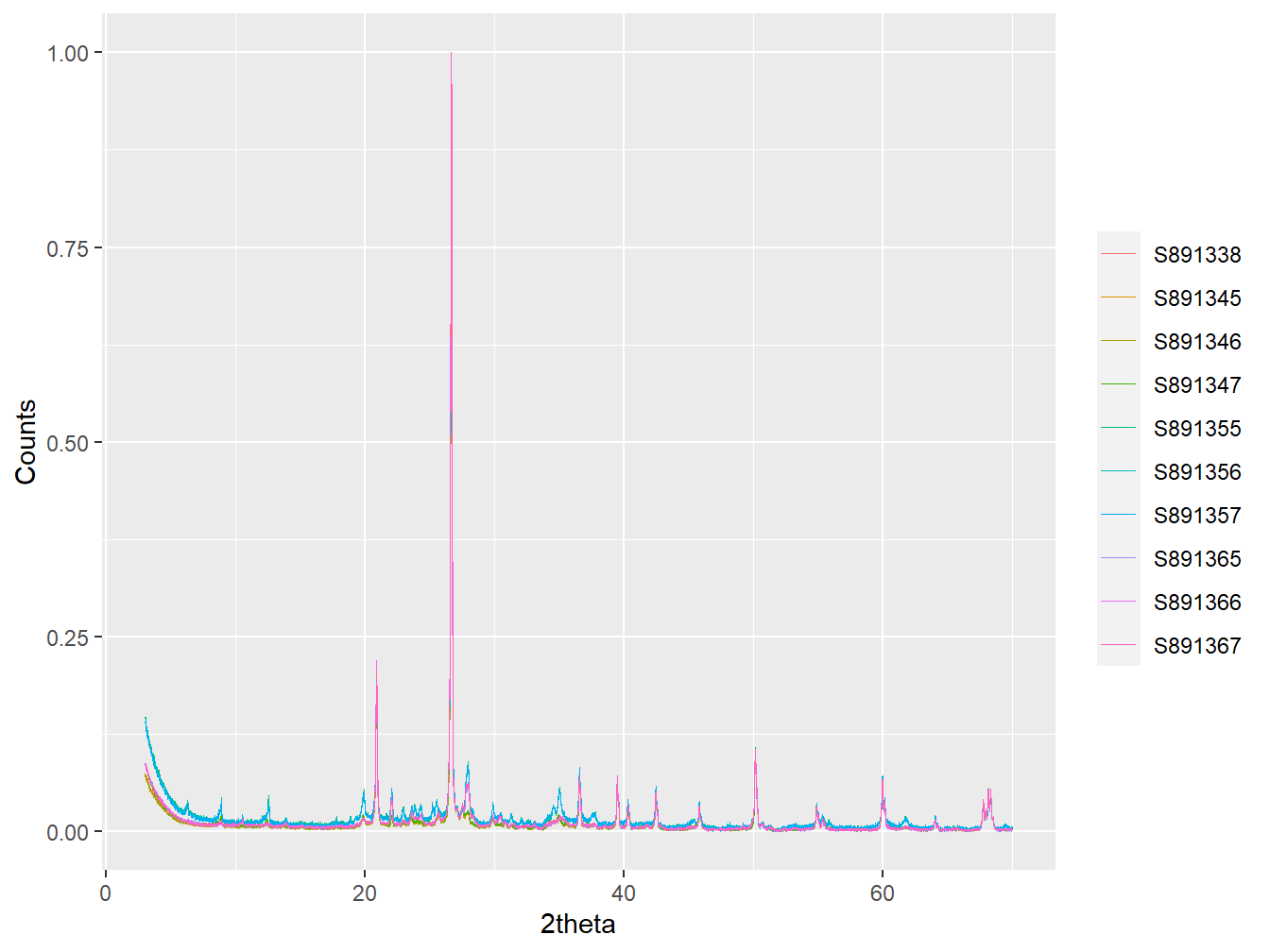
Figure 5.3: The first 10 samples in the scotland_xrpd data.
5.3 Data manipulation
The aim of this analysis is to compare all Martian diffractograms from the MSL to all Scottish soil diffractograms and hence identify those with the greatest similarity. In this case, similarity will be assessed using the Pearson correlation coefficient. Such comparison requires the data to be on identical 2θ axes, which can be achieved by applying the following manipulations to the data:
- Transform the 2θ scale of the
scotland_xrpddata to its Co-Kα equivalent - Interpolate the data onto a harmonised 2θ scale within the overlapping 2θ range
5.3.1 2θ transformation
As outlined here, tth_transform() can be used to transform the 2θ axis of a sample to one that is representative of data recorded using a different wavelength. Here the scotland_xrpd data, which were collected using Cu-Kα radiation, will be transformed to be comparable to the Co-Kα radiation that was used on the MSL diffractometer:
#Convert Scotland_xrpd back to a dataframe for easy alteration of 2theta
scotland_xrpd <- multi_xy_to_df(scotland_xrpd, tth = TRUE)

#Change the 2theta axis
scotland_xrpd$tth <- tth_transform(scotland_xrpd$tth,
                                   from = 1.54056, #Cu-K-alpha wavelength
                                   to = 1.78897) #Co-K-alpha wavelength

#Convert back to multiXY
scotland_xrpd <- as_multi_xy(scotland_xrpd)

#Plot some of the transformed Scotland data
plot(as_multi_xy(scotland_xrpd[1:10]),
     wavelength = "Co",
     normalise = TRUE,
     interactive = FALSE)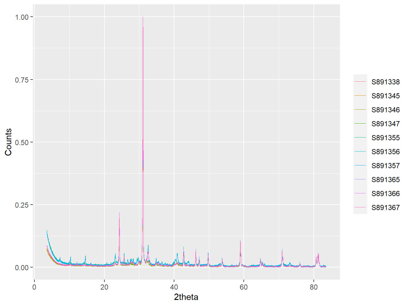
Figure 5.4: The first 10 samples in the scotland_xrpd data after 2theta transformation.
5.3.2 2θ interpolation
Now that the 2θ axis of the scotland_xrpd data is transformed to its Co-Kα equivalent, the overlapping 2θ range of the scotland_xrpd and mars_xrpd data can be computed and used to interpolate all data onto a harmonised 2θ axis:
#Extract the minimum and maximum to use in the harmonised 2theta scale
tth_min <- max(unlist(lapply(c(mars_xrpd, scotland_xrpd), function(x) min(x$tth))))
tth_max <- min(unlist(lapply(c(mars_xrpd, scotland_xrpd), function(x) max(x$tth))))

#Create a new 2theta axis to interpolate all data onto
#using the 0.05 resolution of the MSL data
new_tth <- seq(round(tth_min, 2), round(tth_max, 2), 0.05)

#Interpolate the data
mars_xrpd <- interpolate(mars_xrpd, new_tth)
scotland_xrpd <- interpolate(scotland_xrpd, new_tth)

#Plot some of the transformed and interpolated data
plot(as_multi_xy(scotland_xrpd[1:10]),
     wavelength = "Co",
     normalise = TRUE,
     interactive = FALSE)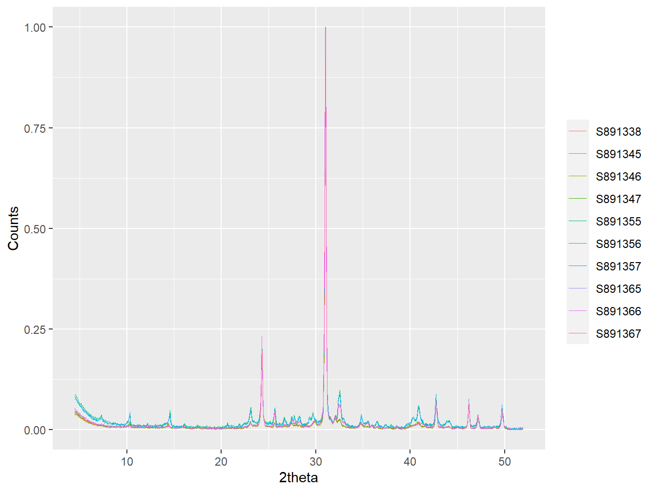
Figure 5.5: The first 10 samples in the scotland_xrpd data following 2theta transformation and interpolation.
5.4 Comparison of XRPD data
Now that the data are harmonised and therefore comparable, the final step is to correlate each MSL diffractogram to every Scottish diffractogram and derive the Pearson correlation coefficients. This comparison should therefore yield 31 vectors each consisting of 703 correlation coefficients (thus 21,793 comparisons in total). In order to further enhance the derived correlation coefficients where similarities are detectable, each pairwise comparison will involve alignment of the 2 samples to one-another in order to correct for common experimental aberrations that can affect peak positions on the 2θ axis. To facilitate this a function will be created that accept the following 3 arguments
marswill be anXYobject of an MSL diffractogram.scotlandwill be anXYobject of a Scottish soil diffractogram.alignwill define the maximum 2θ shift (either positive or negative) that can be applied.
The function will firstly align the two diffractograms to one-another before deriving the Pearson correlation coefficient:
compare_xrpd <- function(mars, scotland, align) {

  #Align the two samples to one another using the multiXY method
  #of the align_xy function
  x <- align_xy(as_multi_xy(list("mars" = mars,
                                 "scotland" = scotland)),
                std = mars,
                xshift = align,
                xmin = min(mars[[1]]),
                xmax = max(mars[[1]]))

  #Correlate the count intensities to one-another
  pearson <- cor(x$mars[[2]], x$scotland[[2]])

  #return the pearson correlation coefficient
  return(pearson)

}
Now that we have created the compare_xrpd() function it will be applied across each of the diffractograms in scotland_xrpd using sapply(). For example, if we wanted to compare every diffractogram in scotland_xrpd to mars_xrpd$Cumberland we could use:
cumberland_to_scotland <- sapply(scotland_xrpd,
                                 compare_xrpd,
                                 mars = mars_xrpd$Cumberland,
                                 align = 0.3
                                 )
Which yields a named vector of 703 correlation coefficients comparing mars_xrpd$Cumberland to every sample within the scotland_xrpd data, with each item within the vector being named according to the sample ID from scotland_xrpd.
#Show the first six values of the names vector
head(cumberland_to_scotland)
## S891338 S891345 S891346 S891347 S891355 S891356
## 0.07680372 0.07571390 0.07945924 0.08710548 0.17750332 0.17151330To derive the correlation coefficients for all 31 samples within the mars_xrpd data instead of just mars$Cumberland, a for loop will be used:
#Create a blank list to populate
mars_to_scotland <- list()

for (i in 1:length(mars_xrpd)) {

  #Use sapply again to derive the named vector of coefficients
  mars_to_scotland[[i]] <- sapply(scotland_xrpd,
                                  compare_xrpd,
                                  mars = mars_xrpd[[i]],
                                  align = 0.3
                                  )

  #name the list item
  names(mars_to_scotland)[i] <- names(mars_xrpd)[i]

}
Which yields a list of 31 named vectors that each take the same form of cumberland_to_scotland. Each item within the list is named according to the MSL site name and consists of 703 numeric correlation coefficients:
summary(mars_to_scotland)## Length Class Mode
## Rocknest_4 703 -none- numeric
## Rocknest_5 703 -none- numeric
## Cumberland 703 -none- numeric
## John_Klein 703 -none- numeric
## Windjana 703 -none- numeric
## Confidence_Hills 703 -none- numeric
## Mojave2 703 -none- numeric
## Telegraph_Peak 703 -none- numeric
## Buckskin 703 -none- numeric
## Big_Sky 703 -none- numeric
## Greenhorn 703 -none- numeric
## Gobabeb_Dune 703 -none- numeric
## Lubango 703 -none- numeric
## Okoruso 703 -none- numeric
## Oudam 703 -none- numeric
## Marimba2 703 -none- numeric
## Quela 703 -none- numeric
## Sebina 703 -none- numeric
## Ogunquit_Beach 703 -none- numeric
## Duluth 703 -none- numeric
## Stoer 703 -none- numeric
## Aberlady 703 -none- numeric
## Kilmarie 703 -none- numeric
## Glen_Etive_1 703 -none- numeric
## Glen_Etive_2 703 -none- numeric
## Hutton 703 -none- numeric
## Edinburgh 703 -none- numeric
## Glasgow 703 -none- numeric
## Mary_Anning_1 703 -none- numeric
## Mary_Anning_3 703 -none- numeric
## Groken 703 -none- numericBy unlisting the mars_to_scotland data using unlist(), we end up with a very long vector consisting of 21,793 correlation coefficients, with each coefficient having a unique name that takes the form MarsSite.ScotlandID.
#Create a vector from the mars_to_scotland list
mars_to_scotland_v <- unlist(mars_to_scotland)

#Check the first correlation coefficient
mars_to_scotland_v[1]
## Rocknest_4.S891338
## 0.1205851with the name {r names(mars_to_scotland_v[1])} detailing that the mars_xrpd$Rocknest_4 and scotland_xrpd$S891338 samples were used to derive this correlation coefficient. It’s possible to plot the aligned data associated with these samples using:
comparison <- align_xy(as_multi_xy(list("Mars_Rocknest_4" = mars_xrpd$Rocknest_4,
                                        "Scotland_S891338" = scotland_xrpd$S891338)),
                       std = mars_xrpd$Rocknest_4,
                       xshift = 0.3,
                       xmin = 4.52,
                       xmax = 51.92)

#Plot the data
plot(comparison,
     wavelength = "Co",
     normalise = TRUE,
     interactive = FALSE)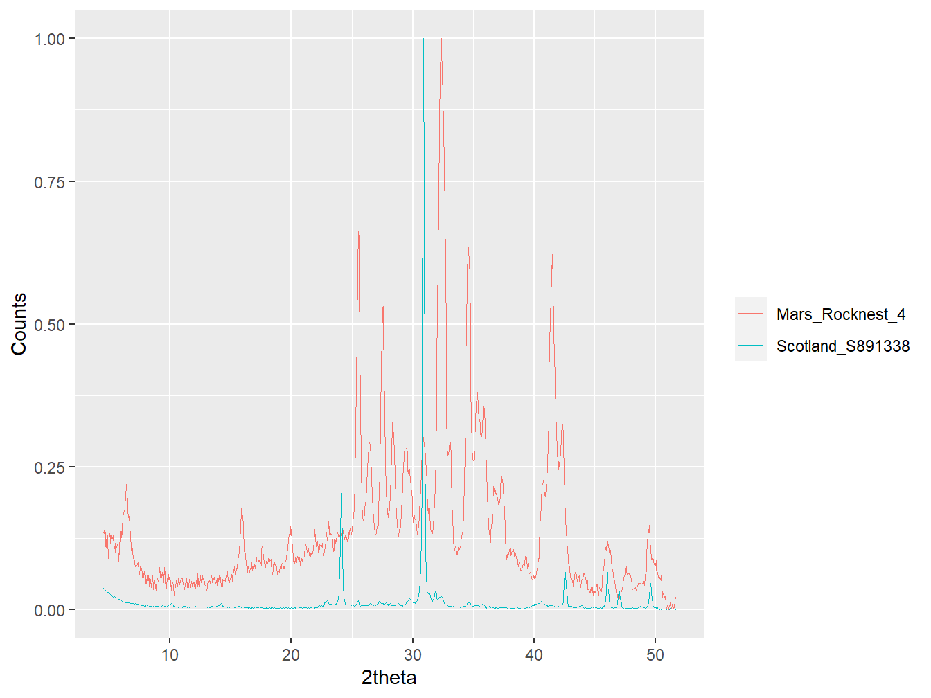
Figure 5.6: Sample Rocknest_4 and S891338 aligned and plotted against one-another.
From this comparison it’s clear to see that these diffractograms are highly dissimilar, which is reflected in their relatively low correlation coefficient of 0.12. However, this is just the first correlation coefficient of ~22,000 that need to be explored, and now that all of the correlation coefficients are in a vector they can easily be summarised and visualised:
#Summarise the correlation coefficients
summary(mars_to_scotland_v)
## Min. 1st Qu. Median Mean 3rd Qu. Max.
## -0.2253 0.1125 0.1681 0.1752 0.2245 0.8091#Produce a histogram of the correlation coefficients
ggplot(data = data.frame("pearson" = mars_to_scotland_v),
aes(x = pearson)) +
geom_histogram(bins = 100, colour = "black", fill = "white") +
xlab("Pearson correlation coefficient") +
ylab("Count")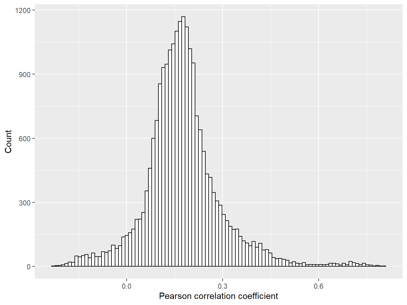
Figure 5.7: Histogram of all 21,793 correlation coefficients
The summary of the data outlines how the correlation coefficients range from -0.2 to 0.8, with an average of ~0.2. The histogram displays an approximately normal distribution of correlation coefficients, but shows a small tail of values >0.75, that can be further explored:
high_cors <- mars_to_scotland_v[mars_to_scotland_v >= 0.75]

#Check the results
high_cors
## Cumberland.S926673 Cumberland.S926674 Cumberland.S968694
## 0.7687338 0.8091307 0.7665140
## John_Klein.S926674 Lubango.S926500 Marimba2.S926499
## 0.7810010 0.7567831 0.7533330
## Marimba2.S968695 Quela.S968695 Sebina.S968695
## 0.8021795 0.7801234 0.7863120
## Duluth.S926674 Aberlady.S926676 Aberlady.S968695
## 0.7522924 0.7530857 0.7752545
## Glen_Etive_2.S926674 Glen_Etive_2.S968694 Glen_Etive_2.S968695
## 0.7610764 0.7585035 0.7974164
## Glasgow.S968695 Mary_Anning_1.S926674 Mary_Anning_1.S968695
## 0.7790987 0.7597717 0.7635760
## Mary_Anning_3.S926674
## 0.7587199#Extract the Mars site names from the high_cors vector
high_cors_mars <- sub("\\..*", "", names(high_cors))
#Show the sites
unique(high_cors_mars)## [1] "Cumberland" "John_Klein" "Lubango" "Marimba2"
## [5] "Quela" "Sebina" "Duluth" "Aberlady"
## [9] "Glen_Etive_2" "Glasgow" "Mary_Anning_1" "Mary_Anning_3"#Extract the Scotland sample IDs from the high cors vector
high_cors_scotland <- sub('.*\\.', '', names(high_cors))
#Show the samples
unique(high_cors_scotland)## [1] "S926673" "S926674" "S968694" "S926500" "S926499" "S968695" "S926676"It’s also possible to plot the samples for each of the sites where high correlations are found. Here we’ll plot the site that displays the highest correlation to samples within the scotland_xrpd dataset:
#Extract the name of the site with the highest correlation coefficients
highest_cor <- sub("\\..*", "", names(high_cors)[which.max(high_cors)])

#print it
highest_cor
## [1] "Cumberland"#Extract the IDs of samples that correlate strongly with Cumberland
scotland_ids <- sub('.*\\.', '', names(high_cors)[grep(highest_cor, names(high_cors))])
#print them
scotland_ids## [1] "S926673" "S926674" "S968694"mars_highest_cor <- as_multi_xy(c(mars_xrpd[highest_cor],
scotland_xrpd[scotland_ids]))
#align data
mars_highest_cor <- align_xy(mars_highest_cor,
std = mars_highest_cor[[1]],
xshift = 0.3,
xmin = 4.52,
xmax = 51.92)
plot(mars_highest_cor,
wavelength = "Co",
normalise = TRUE,
interactive = FALSE)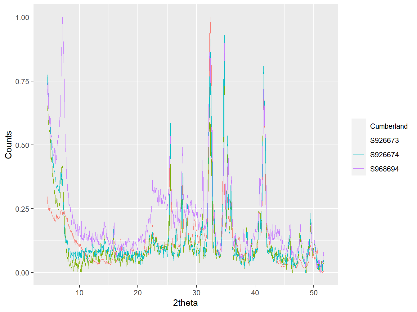
Figure 5.8: Diffractogram from the Cumberland site plotted against 3 diffractograms from Scotland identified as having relatively high correlation to the Martian data.
From this plot (which is best plotted using interactive = TRUE in the function call) we can see how three samples from the scotland_xrpd data show notable similarity to the data from the Cumberland site in the MSL data. Of particular note is the very similar low angle d-spacing of the predominant clay mineral within the samples, suggesting that perhaps similar clay minerals are observed in the samples from Mars and Scotland.
Further exploration of Scottish samples identified as having similar diffraction patterns to the Cumberland MSL sample can be achieved by exploring the data spatially and by understanding more about the parent material that Scottish soils developed from:
leaflet() %>%
  addTiles() %>%
  addCircleMarkers(data = scotland_locations[scotland_locations$SAMPLE_ID %in% scotland_ids,],
                   ~PROFILE_LONGITUDE, ~PROFILE_LATITUDE,
                   color = "blue",
                   opacity = 1)
Figure 5.9: Interactive map of the locations of the Scottish soils that display the highest correlation to samples from the Cumberland MSL site.
Plotting the data spatially reveals that the samples are from two sites that are both located on the West Coast of Scotland. More specifically the sites are on the Isle of Ulva, near the Isle of Mull, and the Trotternish Peninsula on the Isle of Skye. Both of these locations display soils developed from a basaltic parent material in combination with a relatively wet climate that has resulted in the weathering of this material to various clay minerals, which may be useful analogues for Martian clay mineralogy.
In summary, manipulation of XRPD data and data-driven comparisons allows for inter-planetary comparisons of soil samples collected on Earth and Mars. Application of such approaches may serve as a useful way of identifying sites that can be further studied as geological or mineralogy analogues for Mars in order to undertake more detailed analyses that are beyond the capabilities of rover missions.